Managing Security Investment Part III Tyler Moore Computer Science - - PDF document

Managing Security Investment

Part III Tyler Moore

Computer Science & Engineering Department, SMU, Dallas, TX

September 25, 2012

Gordon-Loeb model Baseline models

Outline

1

Gordon-Loeb model Breach probability function Decreasing marginal returns Optimal security investment

2

Baseline models Linear breach probability function Exponential breach probability function Investment models in R

2 / 31 Gordon-Loeb model Baseline models

Review of security investment so far

Metrics for quantifying security benefits

1

ALE0: expected loss without security investment

2

ALEs: expected loss with security investment

3

EBISs: ALE0 − ALEs

4

ENBISs: ALE0 − ALEs − c

High-level investment metrics

1

ROSI

2

NPV

3

IRR

3 / 31 Gordon-Loeb model Baseline models

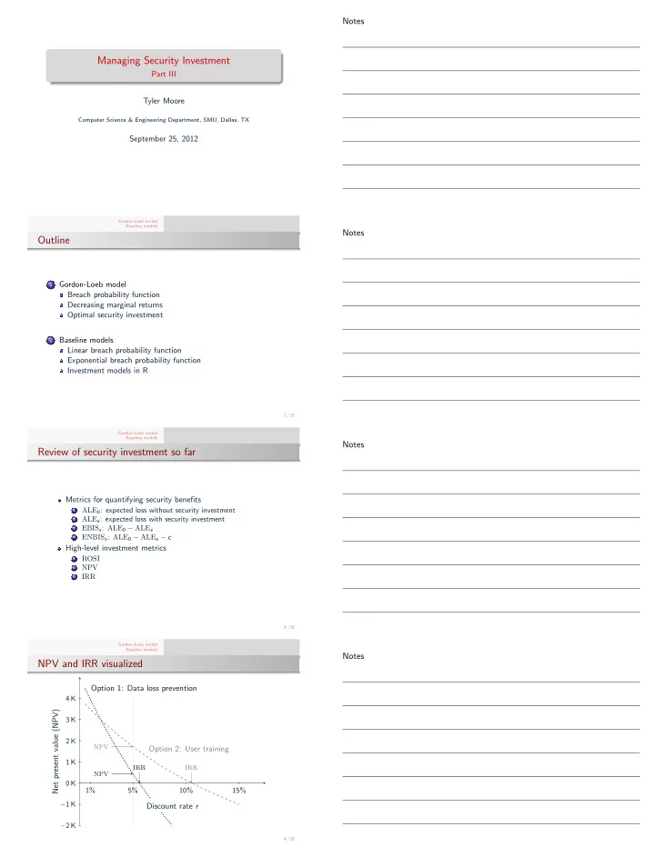
NPV and IRR visualized

Net present value (NPV)

−2 K −1 K 0 K 1 K 2 K 3 K 4 K

Discount rate r

1% 5% 10% 15%

Option 1: Data loss prevention Option 2: User training

NPV NPV IRR IRR

4 / 31

Notes Notes Notes Notes

Gordon-Loeb model Baseline models

Security investment questions worth answering

Q: Should we invest in security? A: Yes, if ENBISs > 0 Q: Should we invest in defense A or B? A: Choose the one with higher ROSI (or NPV if considering longer time horizons) Q: How much should we invest? A: The Gordon-Loeb model can help offer an answer

5 / 31 Gordon-Loeb model Baseline models Breach probability function Decreasing marginal returns Optimal security investment

Gordon-Loeb model

Lawrence Gordon Martin Loeb

7 / 31 Gordon-Loeb model Baseline models Breach probability function Decreasing marginal returns Optimal security investment

Gordon-Loeb model

Model investment decision over a single period Use Bernoulli loss assumption (suffer loss λ with fixed probability ps) The probability of loss depends on two factors: security level and the system’s inherent vulnerability The breach probability function maps these factors to probabilities Gordon and Loeb’s model use assumptions about security investment to derive optimal investment levels based on the breach probability functions

8 / 31 Gordon-Loeb model Baseline models Breach probability function Decreasing marginal returns Optimal security investment

Breach probability function

S : R+ × [0, 1] → [0, 1] Maps a security investment c and an exogenous vulnerability v ∈ [0, 1] to the probability p of incurring a loss of size λ. Furthermore: An invulnerable organization (v = 0) is exposed to no risk regardless of its security investment: p = S(c, 0) = 0 for all c Vulnerability determines the probability of loss of an

• rganization which does not invest in security:

p = S(0, v) = v for all v. S is continuous and twice-differentiable

9 / 31

Notes Notes Notes Notes

Gordon-Loeb model Baseline models Breach probability function Decreasing marginal returns Optimal security investment

Breach probability functions

SI(c, v) = v (αc + 1)β SII(c, v) = vαc+1 α > 0 and β > 1 capture security productivity ⇒ Measure how efficiently the security investment reduces probability of loss Can think of α ∈ (0, 1] as coefficient for linear model relating c to security level s (i.e., s = α · c)

10 / 31 Gordon-Loeb model Baseline models Breach probability function Decreasing marginal returns Optimal security investment

Visualizing SI(c, v) for α = 1

Probability of loss p

1

v = 1

1 2 1 4

Security investment c

1 2 3 4 5

v = 1

2

v = 1

4

β = 5

4

β = 2 SI(c, v) = v (αc + 1)β =

11 / 31 Gordon-Loeb model Baseline models Breach probability function Decreasing marginal returns Optimal security investment

Back to last week’s benefit metrics

EBIS = λ (v − S(c, v)) ENBIS = λ (v − S(c, v)) − c The Gordon-Loeb model assumes that for all v ∈ [0, 1], and all c > 0, S is strictly convex in c, i.e., δc S(c, v) < 0 and δcc S(c, v) > 0

(Note: δc is the first partial derivative with respect to c, and δcc is the second partial derivative with respect to c.)

12 / 31 Gordon-Loeb model Baseline models Breach probability function Decreasing marginal returns Optimal security investment

Decreasing marginal returns to security investment

λv Security investment c v S(c, v) EBIS c1 ∆c ∆EBIS1 c2 ∆c ∆EBIS2

13 / 31

Notes Notes Notes Notes

Gordon-Loeb model Baseline models Breach probability function Decreasing marginal returns Optimal security investment

Why is it reasonable to model security investment with decreasing marginal returns?

In the Gordon-Loeb model, decreasing marginal returns emerge from convexity assumption about S Why is this defensible?

1

Benefits to security are often concave – a rational defender implements the measures with best cost-benefit ratio first, leaving less efficient alternatives if the security budget increases

2

Costs to security are often convex – combining defenses can be more expensive than deploying just one (compatibility issues, management complexity)

Empirical validation (or refutation) of this assumption is an

• pen research question

14 / 31 Gordon-Loeb model Baseline models Breach probability function Decreasing marginal returns Optimal security investment

Choosing an optimal security investment

Given a range of security investment levels, how can a manager choose the optimal amount? If security investment adheres to diminishing marginal returns, then we can identify the investment level c∗ that maximizes the expected net benefit ENBIS

15 / 31 Gordon-Loeb model Baseline models Breach probability function Decreasing marginal returns Optimal security investment

Choosing an optimal security investment

Informally, we look for the investment level where the marginal benefit of security is equal to its marginal cost Formally, we seek the cost level c∗ where: c∗ = max

c

ENBIS(c) We find c∗ using the first-order condition (FOC): δc EBIS(c∗) = 1

16 / 31 Gordon-Loeb model Baseline models Breach probability function Decreasing marginal returns Optimal security investment

Choosing an optimal security investment

We find c∗ using the first-order condition (FOC): δc EBIS(c∗) = 1 δc

• λ(v − S(c∗, v)
• = 1

δc

• λv − λS(c∗, v)
• = 1

−λ δcS(c∗, v) = 1 For c∗ > 0, this condition maximizes ENBIS because EBIS is concave.

17 / 31

Notes Notes Notes Notes

Gordon-Loeb model Baseline models Breach probability function Decreasing marginal returns Optimal security investment

Choosing an optimal security investment, visualized

λv Security investment c EBIS ENBIS = EBIS − c c

45◦

c∗ maxc ENBIS

18 / 31 Gordon-Loeb model Baseline models Breach probability function Decreasing marginal returns Optimal security investment

Gordon-Loeb Rule

The Gordon-Loeb model is very sensitive to values assigned to v: small differences can lead to very different optimal investment levels Furthermore, v can be hard to estimate in practice So they came up with a rule of thumb: never spend more than 37% of your expected loss on security Definition (Gordon–Loeb Rule): The optimal security investment c∗ is bounded from above by λ/e, where e is the base of the natural logarithm.

19 / 31 Gordon-Loeb model Baseline models Linear breach probability function Exponential breach probability function Investment models in R

Other models of security investment are possible

Just because Gordon and Loeb came first doesn’t mean that security investment must be modeled in this way The concavity of security benefits is a nice feature, but might not always apply Simpler breach probability functions could also be used

21 / 31 Gordon-Loeb model Baseline models Linear breach probability function Exponential breach probability function Investment models in R

Linear breach probability function

Let’s start with the simplest possible model

1 We use the Bernoulli loss assumption

Two outcomes {0, λ} 0 : 1 − ps, λ : ps

2 We assume security investment is effective

c = λs For unit loss λ = 1: c = s

3 We can even use a linear breach probability function

S(s, v) = v · (1 − s) for s ∈ [0, 1].

22 / 31

Notes Notes Notes Notes

Gordon-Loeb model Baseline models Linear breach probability function Exponential breach probability function Investment models in R

Linear breach probability function

S(s, v) = v · (1 − s) for s ∈ [0, 1]

0.0 0.2 0.4 0.6 0.8 1.0 0.0 0.2 0.4 0.6 0.8 1.0

Linear breach probability function

Security level s Vulnerability level v v=1 v=1/2 v=1/4

23 / 31 Gordon-Loeb model Baseline models Linear breach probability function Exponential breach probability function Investment models in R

One final simplification

We reduce the action space to just two possibilities – secure (s = 0) and insecure (s = 1) State Security s = c/λ Probability of loss p Expected loss E(λ) Insecure v λv Secure 1 What are the trade-offs between using a linear breach probability function and the one used in the Gordon-Loeb model?

24 / 31 Gordon-Loeb model Baseline models Linear breach probability function Exponential breach probability function Investment models in R

Exponential breach probability function

If diminishing marginal returns is important to include in the model, and we want to retain the Bernoulli loss assumption, then the breach probability function should be convex But the complexity of Gordon-Loeb’s function SI(c, v) =

v (αc+1)β can be hard to justify

We can use a simpler model with one variable for tuning the security productivity instead of two: S(s, v) = vβ−s We require β > 1, and also require S(s, 0) = 0 for all s and S(0, v) = v, as in the Gordon-Loeb model

25 / 31 Gordon-Loeb model Baseline models Linear breach probability function Exponential breach probability function Investment models in R

Exponential breach probability function, visualized

Probability of loss p 1

1 2 1 4

Security level s 1 2 3 4 5 β = 2 β = 8 β = 5

4

v = 1

2

v = 1

26 / 31

Notes Notes Notes Notes

Gordon-Loeb model Baseline models Linear breach probability function Exponential breach probability function Investment models in R

Optimal security investment

We can compute the optimal security investment s∗ using the first-order condition of the ENBIS δs(ENBIS(s∗)) = 0 δs

• v − S(s, v) − s
• = 0

δs

• v − vβ−s − s
• = 0 ,

which has an analytical solution for v > 0: s = log (v log(β)) log(β)

27 / 31 Gordon-Loeb model Baseline models Linear breach probability function Exponential breach probability function Investment models in R

Deriving the optimal security investment condition

δs

• v − vβ−s − s
• = 0

Recall from Calculus class that δx(b−x) = −b−x log b: − v · (−β−s log β) − 1 = 0 β−s = 1 v log β 1 βs = 1 v log β βs = v log β Recall from Algebra class that (i) logb bx = x & (ii) logb x = log x

log b :

log(βs) log(β) = log(v log β) log(β) s = log (v log(β)) log(β)

28 / 31 Gordon-Loeb model Baseline models Linear breach probability function Exponential breach probability function Investment models in R

One more caveat

Some values of β will be negative for the investment condition In particular, s∗ < 0 for β ∈

• 1, e1/v

Consequently, we set the optimal security level as follows: s∗ = max log (v log(β)) log(β) , 0

• If β ∈
• 1, e1/v

, we say that the organization is indefensible The security investment must become more productive to justify any investment

29 / 31 Gordon-Loeb model Baseline models Linear breach probability function Exponential breach probability function Investment models in R

How optimal investment varies

Optimal security level s∗

λ 2 λ 4

Security productivity β

1 5 10 20 30 40 50 60 v = 1 indefensible (v = 1) λ/e (Gordon–Loeb rule of thumb) v = 1

2

indefensible (v = 1

2)

v = 1

4

e2

30 / 31

Notes Notes Notes Notes

Gordon-Loeb model Baseline models Linear breach probability function Exponential breach probability function Investment models in R

Investment models in R

Let’s first review how to make the plot for the linear breach probability function Then let’s explore how optimal investment varies for the exponential breach probability Today’s code: http://lyle.smu.edu/~tylerm/courses/ econsec/code/secinv3.R

31 / 31

Notes Notes Notes Notes