Making Decisions via Simulation Factor Screening [Law, Ch. 10], - PowerPoint PPT Presentation

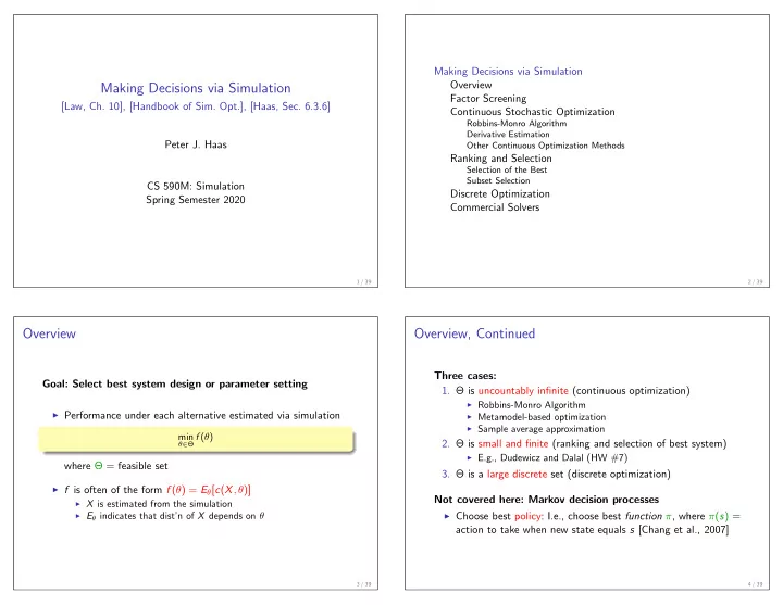
Making Decisions via Simulation Overview Making Decisions via Simulation Factor Screening [Law, Ch. 10], [Handbook of Sim. Opt.], [Haas, Sec. 6.3.6] Continuous Stochastic Optimization Robbins-Monro Algorithm Derivative Estimation Peter J. Haas Other Continuous Optimization Methods Ranking and Selection Selection of the Best Subset Selection CS 590M: Simulation Discrete Optimization Spring Semester 2020 Commercial Solvers 1 / 39 2 / 39 Overview Overview, Continued Three cases: Goal: Select best system design or parameter setting 1. Θ is uncountably infinite (continuous optimization) ◮ Robbins-Monro Algorithm ◮ Performance under each alternative estimated via simulation ◮ Metamodel-based optimization ◮ Sample average approximation min θ ∈ Θ f ( θ ) 2. Θ is small and finite (ranking and selection of best system) ◮ E.g., Dudewicz and Dalal (HW #7) where Θ = feasible set 3. Θ is a large discrete set (discrete optimization) ◮ f is often of the form f ( θ ) = E θ [ c ( X , θ )] Not covered here: Markov decision processes ◮ X is estimated from the simulation ◮ E θ indicates that dist’n of X depends on θ ◮ Choose best policy: I.e., choose best function π , where π ( s ) = action to take when new state equals s [Chang et al., 2007] 3 / 39 4 / 39

Factor Screening Making Decisions via Simulation Overview Factor Screening Continuous Stochastic Optimization Goal: Identify the most important drivers of model response Robbins-Monro Algorithm ◮ Needed for understanding Derivative Estimation ◮ Needed to focus modeling resources (e.g., input distributions) Other Continuous Optimization Methods Ranking and Selection ◮ Needed to select decision variables for optimization Selection of the Best Subset Selection Discrete Optimization Commercial Solvers 5 / 39 6 / 39 Factor Screening, Continued Factor Screening, Continued Based on a simulation metamodel, for example: β i coefficients indicate parameter importance Y ( x ) = β 0 + β 1 x 1 + · · · + β k x k + ǫ 1 0.5 0 ◮ Y = simulation model output -0.5 -1 ◮ Parameters x = ( x 1 , . . . , x k ) 6 ◮ ǫ = noise term (often Gaussian) 4 ◮ Estimate the β i ’s 2 Y(x) 0 using ”low” and ”high” x i values -2 ◮ Test if each | β i | is -4 x1 significantly different from 0 -6 1 0.5 0 -0.5 -1 ◮ Will talk more about metamodels later on... x2 7 / 39 8 / 39

Factor Screening, Continued Factor Screening, Continued Challenge: Many Features Sequential bifurcation ◮ Example with k = 3: ◮ For huge number of factors ◮ Assumes Gaussian noise, nonnegative β ’s β 1 = Y ( h , l , l ) + Y ( h , l , h ) + Y ( h , h , l ) + Y ( h , h , h ) ˆ ◮ Test groups (sums of β i ’s) 4 − Y ( l , l , l ) + Y ( l , l , h ) + Y ( l , h , l ) + Y ( l , h , h ) 4 ◮ In general, need 2 k simulations (”full factorial” design) ◮ Can be smarter, e.g., ”fractional factorial” designs (will talk about this soon) ◮ In general: interplay between metamodel complexity (e.g., β ij terms) and computational cost 9 / 39 10 / 39 Continuous Stochastic Optimization Robbins-Monro Algorithm ◮ Goal: min θ ∈ [ θ,θ ] f ( θ ) Making Decisions via Simulation Overview ◮ Estimate f ′ ( θ ) and use stochastic approximation Factor Screening (also called stochastic gradient descent) Continuous Stochastic Optimization Robbins-Monro Algorithm � a � � � θ n +1 = Π θ n − Z n Derivative Estimation n Other Continuous Optimization Methods where Ranking and Selection Selection of the Best ◮ a > 0 (the gain) Subset Selection ◮ E [ Z n ] = f ′ ( θ n ) Discrete Optimization  Commercial Solvers θ if θ < θ   ◮ Π( θ ) = θ if θ ≤ θ ≤ θ  θ if θ > θ  (projection function) 11 / 39 12 / 39

Continuous Stochastic Optimization, Continued Continuous Stochastic Optimization, Continued Convergence Remarks ◮ Suppose that θ ∗ is true minimizer and the only local minimizer ◮ Variants available for multi-parameter problems ◮ Under mild conditions, lim n →∞ θ n = θ ∗ a.s. ◮ Drawbacks to basic algorithm are slow convergence and high ◮ Q: If θ ∗ is not the only local minimizer, what can go wrong? sensitivity to the gain a ; current research focuses on more ◮ For large n , θ n has approximately a normal dist’n sophisticated methods ◮ Simple improvement: return best value seen so far Estimation Algorithm for 100(1 − δ )% Confidence Interval 1. Fix n ≥ 1 and m ∈ [5 , 10] Kiefer-Wolfowitz algorithm ◮ Replaces derivative f ′ ( θ n ) by finite difference f ( θ n +∆) − f ( θ n − ∆) 2. Run the Robbins-Monro iteration for n steps to obtain θ n 2∆ ◮ Spalls’ simultaneous perturbation stochastic approximation 3. Repeat Step 2 a total of m times to obtain θ n , 1 , . . . , θ n , m (SPSA) method handles high dimensions 4. Compute point estimator ¯ θ m = (1 / m ) � m j =1 θ n , j ◮ At the k th iteration of a d -dimensional problem, run simulation θ m − s m t m − 1 ,δ θ m + s m t m − 1 ,δ 5. Compute 100(1 − δ %) CI as [¯ , ¯ ] √ m √ m at θ k ± c ∆ k , where c > 0 and ∆ k is a vector of i.i.d. random variables I 1 , . . . , I d with P ( I j = 1) = P ( I j = − 1) = 0 . 5 θ ) 2 and t m − 1 ,δ = Student-t quantile � m j =1 ( θ n , j − ¯ where s 2 1 m = m − 1 13 / 39 14 / 39 Estimating the Derivative f ′ ( θ n ) Suppose that f ( θ ) = E θ [ c ( X , θ )] ◮ Ex: M/M/1 queue with interarrival rate λ and service rate θ Making Decisions via Simulation ◮ X = average waiting time for first 100 customers Overview ◮ c ( x , θ ) = a θ + bx (trades off operating costs and delay costs) Factor Screening Use likelihood ratios Continuous Stochastic Optimization ◮ We have f ( θ + h ) = E θ + h [ c ( X , θ + h )] = E θ [ c ( X , θ + h ) L ( h )] Robbins-Monro Algorithm Derivative Estimation for appropriate likelihood L ( h ) Other Continuous Optimization Methods Ranking and Selection f ( θ + h ) − f ( θ ) f ′ ( θ ) = lim Selection of the Best h h → 0 Subset Selection � c ( X , θ + h ) L ( h ) − c ( X , θ ) L (0) � = lim h → 0 E θ Discrete Optimization h Commercial Solvers c ( X , θ + h ) L ( h ) − c ( X , θ ) L (0) � � = E θ lim under regularity cond. h h → 0 � d � � � � = E θ c ( X , θ + h ) L ( h ) � dh � h =0 c ′ = ∂ c /∂θ L ′ = ∂ L /∂ h � c ′ ( X , θ ) + c ( X , θ ) L ′ (0) � = E θ 15 / 39 16 / 39

Derivative Estimation, Continued Derivative Estimation, Continued Ex: M/M/1 queue To estimate g ( θ ) ∆ = f ′ ( θ ) = E θ � c ′ ( X , θ ) + c ( X , θ ) L ′ (0) � ◮ Let V 1 , . . . , V 100 be the 100 generated service times ◮ Simulate system to generate i.i.d. replicates X 1 , . . . , X m ◮ Let X = avg of the 100 waiting times (the perf. measure) ◮ At the same time, compute L ′ 1 (0) , . . . , L ′ m (0) � m ◮ Compute the estimate g m ( θ ) = 1 i =1 [ c ′ ( X i , θ ) + c ( X i , θ ) L ′ i (0)] 100 100 ( θ + h ) e − ( θ + h ) V i � θ + h � m � � e − hV i L ( h ) = = ◮ Robbins and Monro showed that taking m = 1 is optimal θ e − θ V i θ i =1 i =1 (many approximate steps vs few precise steps) 100 � 1 � � ⇒ L ′ (0) = θ − V i (can be computed incrementally) i =1 n th step of R-M algorithm 1. Generate a single sample X of the performance measure c ( x , θ ) = a θ + bx ⇒ c ′ ( x , θ ) = a and compute L ′ (0) 2. Set Z n = g 1 ( θ n ) = c ′ ( X , θ n ) + c ( X , θ n ) L ′ (0) � a � � � � 1 100 3. Set θ n +1 = Π θ n − Z n � � Z n = c ′ ( X n , θ n ) + c ( X n , θ n ) L ′ n (0) = a + ( a θ n + bX n ) − V n , i n θ n i =1 17 / 39 18 / 39 Derivative Estimation, Continued Derivative Estimation, Continued A trick for computing L ′ (0) ◮ Likelihood ratio often has form: L ( h ) = r 1 ( h ) r 2 ( h ) · · · r k ( h ) P θ + h ( S j +1 ; S j , e ∗ j ) ◮ E.g., for a GSMP, r i ( h ) = f θ + h ( X ; s ′ , e ′ , s , e ∗ ) Trick continued: M/M/1 queue or f θ ( X ; s ′ , e ′ , s , e ∗ ) P θ ( S j +1 ; S j , e ∗ j ) ◮ Using the product rule and the fact that r i (0) = 1 for all i 100 100 f θ + h ( V i ) � � L ( h ) = r i ( h ) = d h =0 = d � �� f θ ( V i ) � dhL ( h ) r 1 ( h ) r 2 ( h ) · · · r k ( h ) � � i =1 i =1 � dh � h =0 r 1 ( h ) d � � �� � � = r 2 ( h ) · · · r k ( h ) h =0 + r ′ 1 ( h ) r 2 ( h ) · · · r k ( h ) f θ ( v ) = θ e − θ v θ ( v ) = (1 − θ v ) e − θ v f ′ and h =0 dh = d � � h =0 + r ′ r 2 ( h ) · · · r k ( h ) 1 (0) dh 100 100 100 (1 − θ V i ) e − θ V i f ′ θ ( V i ) � 1 � � � � L ′ (0) = f θ ( V i ) = = θ − V i ◮ By induction: L ′ (0) = r ′ 1 (0) + · · · + r ′ k (0) θ e − θ V i i =1 i =1 i =1 (compute incrementally) ◮ For GSMP example (with f ′ θ = ∂ f θ /∂θ ): d � dh f θ + h ( X ; s ′ , e ′ , s , e ∗ ) = f ′ θ ( X ; s ′ , e ′ , s , e ∗ ) � h =0 r ′ i (0) = f θ ( X ; s ′ , e ′ , s , e ∗ ) f θ ( X ; s ′ , e ′ , s , e ∗ ) 19 / 39 20 / 39