Low-Cost Learning via Active Data Procurement October 2015 Jacob - - PowerPoint PPT Presentation

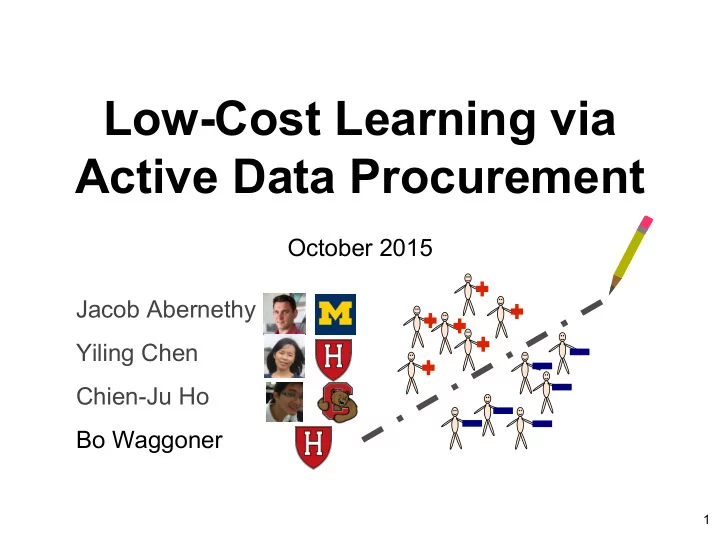
Low-Cost Learning via Active Data Procurement

October 2015 Jacob Abernethy Yiling Chen Chien-Ju Ho Bo Waggoner

1

2

Coming soon to a society near you

d a t a

• h
• l

d e r s ex: medical data data-needers ex: pharmaceutical co.

3

Classic ML problem

z1 z2

learning alg

data source h

hypothesis data data-needer Goal: use small amount of data, output “good” h.

4

Example learning task: classification

• Data: (point, label) where label is or
• Hypothesis: hyperplane separating the two types

h

h

5

Twist: data is now held by individuals

c1 z1 z2

mechanism

data source

c2

h

hypothesis “Cost of revealing data” (formal model later…) Goal: spend small budget, output “good” h. data-needer data-holders

6

Why is this difficult?

• 1. (Relatively) few data are useful

Studying ACTN-3 mutation and endurance running have mutation runners

7

Why is this difficult?

• 2. Utility of data may be correlated with cost (causing bias)

Paying $10 for data (to study HIV) HIV-negative yes yes no yes yes HIV-positive no no yes

8

Why is this difficult?

• 2. Utility of data may be correlated with cost (causing bias)

Paying $10 for data (to study HIV) HIV-negative yes yes no yes yes HIV-positive no no yes

Machine Learning roadblock: how to deal with biases?

9

Why is this difficult?

• 3. Utility (ML) and cost (econ) live in different worlds

learning alg

entropies, gradients, loss functions, divergences

mechanism

auctions, budgets, value distributions, reserve prices

10

Why is this difficult?

• 3. Utility (ML) and cost (econ) live in different worlds

learning alg

entropies, gradients, loss functions, divergences

mechanism

auctions, budgets, value distributions, reserve prices

Econ roadblock: how to assign value to data?

11

Broad research challenge:

• 1. How to assign value (prices) to pieces of data?
• 2. How to design mechanisms for procuring and

learning from data?

• 3. Develop a theory of budget-constrained learning:

what is (im)possible to learn given budget B and parameters of the problem?

12

Outline

• 1. Overview of literature,
• ur contributions
• 2. Online learning model/results
• 3. “Statistical learning” result,

conclusion

13

Related work

Cummings, Ligett, Roth, Wu, Ziani 2015 Horel, Ionnadis, Muthukrishnan 2014 Roth, Schoenebeck 2012 Ligett, Roth 2012 Cai, Daskalakis, Papadimitriou 2015 principal-agent style, data depends on effort agents cannot fabricate data, have costs this work

How are agents strategic?

14

Related work

Cummings, Ligett, Roth, Wu, Ziani 2015 Horel, Ionnadis, Muthukrishnan 2014 Roth, Schoenebeck 2012 Ligett, Roth 2012 Cai, Daskalakis, Papadimitriou 2015 principal-agent style, data depends on effort agents cannot fabricate data, have costs this work

minimize variance

• r related goal

risk/regret bounds Type of goal

15

Related work

Cummings, Ligett, Roth, Wu, Ziani 2015 Horel, Ionnadis, Muthukrishnan 2014 Roth, Schoenebeck 2012 Ligett, Roth 2012 Cai, Daskalakis, Papadimitriou 2015 principal-agent style, data depends on effort agents cannot fabricate data, have costs this work

minimize variance

• r related goal

risk/regret bounds

Waggoner, Frongillo, Abernethy NIPS 2015: prediction-market style mechanism

Conducting Truthful Surveys, Cheaply

• Each datapoint is a number. Task is to estimate the mean
• Approach: offer each agent a price drawn i.i.d.
• Goal: minimize the estimate’s variance

16

e.g. Roth-Schoenebeck, EC 2012

c1 1

data source

c2

h

i.i.d.

17

What we wanted to do differently

• 1. Prove ML-style risk or regret bounds

Why: ML-style approach: understand error rate as function of budget and problem characteristics.

• 2. Interface with existing ML algorithms.

Why: understand how value derives from learning alg. Toward black-box use of learners in mechanisms.

• 3. Online data arrival

Why: active-learning approach, simpler model

18

Overview of our contributions

Propose model of online learning with purchased data: T arriving data points and budget B. Convert any “FTRL” algorithm into a mechanism. Show regret on order of T / √B and lower bounds of same order.

Extend model to case where data is drawn i.i.d. (“statistical learning”) Extend result to “risk” bound on order of 1 / √B .

19

Overview of our contributions

Propose model of online learning with purchased data: T arriving data points and budget B. Convert any “FTRL” algorithm into a mechanism. Show regret on order of T / √B and lower bounds of same order.

20

Outline

• 1. Overview of literature,
• ur contributions
• 2. Online learning model/results
• 3. “Statistical learning” result,

conclusion

21

Online learning with purchased data

• a. Review of online learning
• b. Our model: adding $$
• c. Deriving our mechanism

and results

22

Standard online learning model

For t = 1, …, T:

• algorithm posts a hypothesis ht
• data point zt arrives
• algorithm sees zt and updates to ht+1

Loss = ∑t ℓ(ht, zt) Regret = Loss - ∑t ℓ(h*, zt)

where h* minimizes sum

23

Follow-the-Regularized-Leader (FTRL)

Assume: loss function is convex and Lipschitz, hypothesis space is Hilbert, etc

Algorithm: ht = argmin ∑s<t ℓ(h, zs) + R(h)/η

24

Follow-the-Regularized-Leader (FTRL)

Assume: loss function is convex and Lipschitz, hypothesis space is Hilbert, etc

Algorithm: ht = argmin ∑s<t ℓ(h, zs) + R(h)/η Example 1 (Euclidean norm): R(h) = ǁhǁ2

2

⇒ ht = ht-1 - η∇ℓ(h, zt)

• nline gradient descent

25

Follow-the-Regularized-Leader (FTRL)

Assume: loss function is convex and Lipschitz, hypothesis space is Hilbert, etc

Algorithm: ht = argmin ∑s<t ℓ(h, zs) + R(h)/η Example 1 (Euclidean norm): R(h) = ǁhǁ2

2

⇒ ht = ht-1 - η∇ℓ(h, zt)

• nline gradient descent

Example 2 (negative entropy): R(h) = ∑j h(j) ln(h(j)). ⇒ ht

(j) ∝ ht-1 (j) exp[ η∇ℓ(ht-1, zt ) ]

multiplicative weights

26

Regret Bound for FTRL

Fact: the regret of FTRL is bounded by O of 1/η + η ∑t Δt

2 where Δt = ǁ ∇ℓ(ht, zt) ǁ.

27

Regret Bound for FTRL

Fact: the regret of FTRL is bounded by O of 1/η + η ∑t Δt

2 where Δt = ǁ ∇ℓ(ht, zt) ǁ.

We know Δt ≤ 1 by assumption, so we can choose η=1/√T and get Regret ≤ O(√T ). “No regret”: average regret → 0.

28

Online learning with purchased data

• a. Review of online learning
• b. Our model: adding $$
• c. Deriving our mechanism

and results

29

First: model of strategic data-holder

Model of agent:

• holds data zt and cost ct
• cost is threshold price

○ agent agrees to sell data iff price ≥ ct ○ interpretations: privacy, transaction cost, ….

• Assume: all costs ≤ 1

ct zt

30

Model of agent-mechanism interaction

• Mechanism posts menu of prices offered:
• agent t arrives
• If ct ≤ price(zt), agent accepts:

○ agent reveals (zt, ct) ○ mechanism pays agent price(zt)

• Otherwise, agent rejects:

○ mechanism learns that agent rejected, pays nothing

data: (32,12) (20,18) (32,12) price: $0.22 $0.41 $0.88

ct zt

31

Recall: standard online learning model

For t = 1, …, T:

• algorithm posts a hypothesis ht
• data point zt arrives
• algorithm sees zt and updates to ht+1

32

Our model: online learning with $$

For t = 1, …, T:

• mechanism posts a hypothesis ht

and a menu of prices

• data point zt arrives with cost ct
• If ct ≤ menu price of zt: mech pays price, learns zt
• else: mech pays nothing

Loss = ∑t ℓ(ht, zt) Regret = Loss - ∑t ℓ(h*, zt)

where h* minimizes sum

ct zt

33

Online learning with purchased data

• a. Review of online learning
• b. Our model: adding $$
• c. Deriving our mechanism

and results

34

Start easy

Suppose all costs are 1. ⇒ Determine which data points to sample.

ct zt

data: (32,12) (20,18) (32,12) price: $1 $0 $0

35

Start easy

Suppose all costs are 1. ⇒ Determine which data points to sample. Examples:

• B = T/2
• B = √T
• B = log(T)

ct zt

data: (32,12) (20,18) (32,12) price: $1 $0 $0

36

Key idea #1: randomly sample

Can purchase each data point zt with probability qt(zt). Menu is now randomly chosen:

data: (32,12) (20,18) (32,12) Pr[price=1]: 0.3 0.06 0.41

1/η + E [ η ∑t (Δt

2 / qt) ]

37

Key idea #1: randomly sample

Can purchase each data point zt with probability qt(zt). Menu is now randomly chosen:

data: (32,12) (20,18) (32,12) Pr[price=1]: 0.3 0.06 0.41

Lemma (importance-weighted regret bound): For any qts, the regret of (modified) FTRL is O of 1/η + η E [ ∑t (Δt

2 / qt) ]

See also: Importance-Weighted Active Learning, Beygelzimer et al, ICML 2009.

38

Result for easy case

Lemma (importance-weighted regret bound): For any qts, the regret of (modified) FTRL is O of Corollary: Setting all qt = B/T and choosing η =√B / T yields regret ≤ T / √B . 1/η + η E [ ∑t (Δt

2 / qt) ]

“No data, no regret”: average amount of data → 0 and average regret → 0.

39

Result for easy case

Lemma (importance-weighted regret bound): For any qts, the regret of (modified) FTRL is O of Corollary: Setting all qt = B/T and choosing η =√B / T yields regret ≤ T / √B . Theorem: This is tight.

(Predict a repeated coin toss whose bias is either 1+1/√B or 1-1/√B )

1/η + η E [ ∑t (Δt

2 / qt) ]

40

Now a bit harder….

Costs can be arbitrary, but agents are nonstrategic: they will accept payment exactly ct. At each time step, randomly choose which (data, cost) pairs to purchase. Question: how to set probabilities of purchase qt?

data,cost: (32,12) , c=0.3 (20,18) , c=0.8 Pr[purchase]: 0.12 0.08

41

Key idea #2: sample proportional to...

Imagine we knew the arrivals in advance. Optimization problem: minimize ∑t (Δt

2 / qt)

s.t. ∑t qt ct ≤ B qt ≤ 1. Solution: qt = Δt

/ K √ct (K a normalizing constant).

ct zt

42

Key idea #2: sample proportional to...

Imagine we knew the arrivals in advance. Optimization problem: minimize ∑t (Δt

2 / qt)

s.t. ∑t qt ct ≤ B qt ≤ 1. Solution: qt = Δt

/ K √ct (K a normalizing constant).

The point: only need advance knowledge of K to implement the “optimal” sampling strategy! Turns out: K = T / B, where ∈ [0,1] (discuss later)

ct zt

43

Result for this “at-cost” setting

Theorem: Given rough advance estimate of , can achieve regret ≤ T / √B Theorem: This is tight (in a reasonable sense).

(Same bad instance, but with “useless” free data points sprinkled in.)

Implication: is capturing the “difficulty of the problem”.

= (1/T) ∑t Δt √ct = average sqrt(difficulty * cost).

44

Discussion

= (1/T) ∑t Δt √ct = average sqrt(difficulty * cost).

• Low avg cost ⇒ low regret
• Low avg difficulty ⇒ low regret
• good correlations ⇒ low regret

45

Discussion

Example simplified corollary: Given rough advance estimate of avg cost μ, regret ≤ √μ T / √B

46

Finally, the “full” problem.

ct zt

Now agents are strategic and we must post prices. Recall: had sampling probability qt = Δt

/ K √ct .

But: we don’t know ct.

47

Finally, the “full” problem.

ct zt

Now agents are strategic and we must post prices. Recall: had sampling probability qt = Δt

/ K √ct .

But: we don’t know ct. Key idea #3: randomly draw price from the distribution s.t. Pr[ price ≥ ct] = Δt

/ K √ct .

⇒ achieve the “right” probability for every ct simultaneously!

48

Description of final mechanism

Input: estimate of At each time t:

• post hypothesis ht ← FTRL
• for each data point zt, compute Δt = ǁ ∇ℓ(ht, zt) ǁ

and post random price from distribution

• If arriving agent accepts,

send “re-weighted” zt → FTRL

49

Main result for online learning setting

Theorem: Given rough advance estimate of , can achieve Theorem (recall): No mechanism for the easier, “at-cost” setting can beat regret ≤ T / √B regret ≤ √ T / √B Note: lost a √ factor compared to easier setting, due to paying our posted price rather than the agent’s cost. (“cost of strategic behavior”)

50

Outline

• 1. Overview of literature,
• ur contributions
• 2. Online learning model/results
• 3. “Statistical learning” result,

conclusion

Extend model to case where data is drawn i.i.d. (“statistical learning”) Extend result to “risk” bound on order of 1 / √B .

51

Recalling contributions

Propose model of online learning with purchased data: T arriving data points and budget B. Convert any “FTRL” algorithm into a mechanism. Show regret on order of T / √B and lower bounds of same order.

52

Classic statistical learning model

For classification:

E loss( h ) ≤ E loss( h* ) + O

VC-dim

T

z1 z2

learning alg

data source h

hypothesis i.i.d.

53

Our statistical learning model

c1 z1 z2

mechanism

data source

c2

h

hypothesis i.i.d.

• B

costs (still) may be adversarially chosen

54

Our statistical learning model

c1 z1 z2

mechanism

data source

c2

h

hypothesis i.i.d. Theorem: Given rough advance estimate of , can achieve

E loss( h ) ≤ E loss( h* ) + O

• B

55

Our statistical learning model

c1 z1 z2

mechanism

data source

c2

h

hypothesis i.i.d. Theorem: Given rough advance estimate of , can achieve

E loss( h ) ≤ E loss( h* ) + O

• B

Proof: known “online-to-batch conversion”: regret R ⇒ risk R/T

56

Summary

Model:

• online arrival of agents
• post prices to procure data
• adversarial costs and data

(online learning setting)

• adversarial costs, i.i.d. data

(statistical learning setting)

57

Summary

Results:

• upper/lower bounds on regret

(online learning setting)

• upper bound on risk

(statistical learning setting)

58

Summary

Big picture:

• design mechanisms to interface with existing

learning algs

• prove ML-style bounds: risk and regret
• toward a “theory of the learnable...on a budget”

59

Future work

• Improve bounds (!)
• Propose “universal quantity” to replace

γ in bounds (analogue of VC-dimension?)

• Explore models for purchasing data

60

Future work

• Improve bounds (!)
• Propose “universal quantity” to replace

γ in bounds (analogue of VC-dimension?)

• Explore models for purchasing data

Thanks!

Additional slides

61

62

Simulation results

MNIST dataset -- handwritten digit classification Brighter green = higher cost Toy problem: classify (1 or 4) vs (9 or 8)

63

Simulation results

• T = 8503
• train on half,

test on half

• Alg: Online Gradient

Descent Naive: pay 1 until budget is exhausted, then run alg Baseline: run alg on all data points (no budget) Large γ: bad correlations Small γ: independent cost/data

64

Pricing distribution