Logistic Regression Lecture 6 Logistic Regression Classification - PDF document

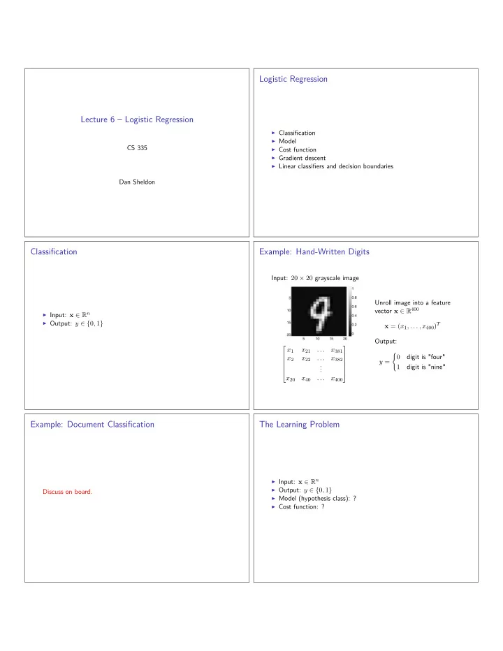
Logistic Regression Lecture 6 – Logistic Regression ◮ Classification ◮ Model CS 335 ◮ Cost function ◮ Gradient descent ◮ Linear classifiers and decision boundaries Dan Sheldon Classification Example: Hand-Written Digits Input: 20 × 20 grayscale image Unroll image into a feature vector x ∈ R 400 ◮ Input: x ∈ R n ◮ Output: y ∈ { 0 , 1 } x = ( x 1 , . . . , x 400 ) T Output:   x 1 x 21 . . . x 381 � 0 digit is "four" x 2 x 22 . . . x 382   y =   .   1 digit is "nine" . .     x 20 x 40 . . . x 400 Example: Document Classification The Learning Problem ◮ Input: x ∈ R n ◮ Output: y ∈ { 0 , 1 } Discuss on board. ◮ Model (hypothesis class): ? ◮ Cost function: ?

Classification as regression? The Model Exercise: fix the linear regression model Discuss on board h θ ( x ) = g ( θ T x ) , g : R → [0 , 1] . What should g look like? Logistic Function The Model 1 Put it together g ( z ) = 1 + e − z 1 h θ ( x ) = logistic( θ T x ) = 1 1 + e − θ T x g(z) 0.5 0 Nuance: −20 −15 −10 −5 0 5 10 15 20 z ◮ Output is in [0 , 1] , not { 0 , 1 } . ◮ This is called the logistic or sigmoid function ◮ Interpret as probability g ( z ) = logistic( z ) = sigmoid( z ) Hypothesis vs. Prediction Rule Prediction Rule 1 Hypothesis (for learning, or when probability is useful) y 0.5 1 0 h θ (x) 0.5 −20 −15 −10 −5 0 5 10 15 20 θ T x Rule 0 −20 −15 −10 −5 0 5 10 15 20 θ T x � 0 if h θ ( x ) < 1 / 2 Prediction rule (when you need to commit!) y = 1 if h θ ( x ) ≥ 1 / 2 1 Equivalent rule 0.5 y � if θ T x < 0 0 0 y = −20 −15 −10 −5 0 5 10 15 20 if θ T x ≥ 0 . 1 θ T x

The Model—Big Picture Cost Function Can we used squared error? Illustrate on board: x → z → p → y � ( h θ ( x ( i ) ) − y ( i ) ) 2 J ( θ ) = MATLAB visualization i This is sometimes done. But we want to do better. Cost Function Cost Function Suppose y = 1 . For squared error, cost( p, 1) looks like this 1 0.8 Let’s explore further. For squared error, we can write: squared error 0.6 m 0.4 � cost( h θ ( x ( i ) ) , y ( i ) ) J ( θ ) = 0.2 i =1 0 0 0.2 0.4 0.6 0.8 1 cost( p, y ) = ( p − y ) 2 h(x) If we undo the logistic transform, it looks like this cost( p, y ) is cost of predicting h θ ( x ) = p when the true value is y 1 squared error 0.5 0 −20 −10 0 10 20 θ T x Cost Function Log Loss ( y = 1) Exercise: fix these 1 cost ( p, 1) = − log p 0.8 squared error 0.6 5 0.4 4 0.2 log loss 3 0 0 0.2 0.4 0.6 0.8 1 h(x) 2 1 squared error 1 0.5 0 0 0 0.2 0.4 0.6 0.8 1 −20 −10 0 10 20 h(x) θ T x ◮ Recall that y = 1 is the correct answer 20 log loss ◮ As z = θ T x → ∞ , then p → 1 , so the prediction is better and better. 10 The cost approaches zero. ◮ As z = θ T x → −∞ , then p → 0 , so the prediction is worse and worse. 0 −20 −10 0 10 20 The cost. . . θ T x

Log Loss Equivalent Expression for Log-Loss � − log p y = 1 � − log p y = 1 cost ( p, y ) = cost ( p, y ) = − log(1 − p ) y = 0 − log(1 − p ) y = 0 5 y=1 y=0 4 cost ( p, y ) = − y log p − (1 − y ) log(1 − p ) log loss 3 y=1 20 log loss y=0 2 10 1 cost ( h θ ( x ) , y ) = − y log h θ ( x ) − (1 − y ) log(1 − h θ ( x )) 0 0 −20 −10 0 10 20 0 0.2 0.4 0.6 0.8 1 θ T x h(x) Review so far Gradient Descent for Logistic Regression ◮ Input: x ∈ R n 1. Initialize θ 0 , θ 1 , . . . , θ d arbitrarily ◮ Output: y ∈ { 0 , 1 } 2. Repeat until convergence ◮ Model (hypothesis class) 1 θ j ← θ j − α ∂ h θ ( x ) = logistic ( θ T x ) = J ( θ ) , j = 0 , . . . , d. 1 + e − θ T x ∂θ j ◮ Cost function: Partial derivatives for logistic regression (exercise): m ∂ ( h θ ( x ( i ) ) − y ( i ) ) x ( i ) m � J ( θ ) = 2 � − y ( i ) log h θ ( x ( i ) ) − (1 − y ( i ) ) log(1 − h θ ( x ( i ) )) � � j J ( θ ) = ∂θ j i =1 i =1 (Same as linear regression! But h θ ( x ) is different ) TODO: optimize J ( θ ) Decision Boundaries Decision Boundaries 7.5 7 6.5 Example from R&N (Fig. 18.15). 6 5.5 5 7.5 x 2 7 4.5 4 6.5 6 3.5 3 5.5 5 2.5 x 2 4.5 4.5 5 5.5 6 6.5 7 4 x 1 3.5 E.g., suppose hypothesis is 3 2.5 4.5 5 5.5 6 6.5 7 h ( x 1 , x 2 ) = logistic (1 . 7 x 1 − x 2 − 4 . 9) x 1 Figure 1: Earthquakes (white circles) vs. nuclear explosions (black circles) Predict nuclear explosion if: by body wave magnitude ( x 1 ) and surface wave magnitude ( x 2 ) 1 . 7 x 1 − x 2 − 4 . 9 ≥ 0 x 2 ≤ 1 . 7 x 1 − 4 . 9

Linear Classifiers Nonlinear Decision Boundaries by Feature Expansion Example (Ng) Predict ( x 1 , x 2 ) �→ (1 , x 1 , x 2 , x 2 1 , x 2 � if θ T x < 0 , 2 , x 1 x 2 ) , 0 y = if θ T x ≥ 0 . � T 1 � θ = − 1 0 0 1 1 0 Exercise: what does decision boundary look like in ( x 1 , x 2 ) plane? Watch out! Hyperplane! Many other learning algorithms use linear classification rules ◮ Perceptron ◮ Support vector machines (SVMs) ◮ Linear discriminants Note: Where Does Log Loss Come From? � p y = 1 probability of y given p = 1 − p y = 0 � − log p y = 1 cost( p, y ) = − log probability = − log(1 − p ) y = 0 Find θ to minimize cost ← → Find θ to maximize probability