Linear and Logistic Regression Marta Arias marias@cs.upc.edu Dept. - PowerPoint PPT Presentation

Linear and Logistic Regression Marta Arias marias@cs.upc.edu Dept. CS, UPC Fall 2018

Linear regression Linear models y = a 1 ∗ x 1 + a 2 ∗ x 2 + ... + b x i are the attributes, y is the target value a i and b are the coefficients or parameters of the linear model For example: house _ price = 2 ∗ area + 0.5 ∗ proximity _ metro + 150 or house _ price = 25 ∗ area − 0.5 ∗ proximity _ metro + 1500

Linear regression Example: housing prices area price 300 x i y i i 200 1 60 120 price 2 80 150 100 3 100 180 50 4 120 250 0 110 ? 60 80 100 120 140 squared meters

Linear regression Example: housing prices

Linear regression Example: housing prices area price 300 x i y i i 200 1 60 120 price 2 80 150 100 3 100 180 50 4 120 250 0 110 ? 60 80 100 120 140 squared meters Want to find the line that best fits the available data find parameters a and b such that ax i + b is closest to y i (for all i simultaneously), e.g. minimize squared error : � ( ax i + b − y i ) 2 arg min a , b i

Linear regression Example: housing prices area price 300 x i y i i 200 1 60 120 price 2 80 150 100 3 100 180 50 4 120 250 0 110 ? 60 80 100 120 140 squared meters In this case, we seek parameters ( a , b ) that minimize J ( a , b ) = � i ( ax i + b − y i ) 2 ( 60 a + b − 120 ) 2 J ( a , b ) = J ( a = 2.1, b = − 14 ) = 480 ( 80 a + b − 150 ) 2 + J ( a = 2.1, b = − 10 ) = 544 ( 100 a + b − 180 ) 2 + J ( a = 2.0, b = − 14 ) = 824 ( 120 a + b − 250 ) 2 + J ( a = − 2.1, b = − 14 ) = 607296

Linear regression Simple case: R 2 Here is the idea: 1. Got a bunch of points in R 2 , { ( x i , y i ) } . 2. Want to fit a line y = ax + b that describes the trend. 3. We define a cost function that computes the total squared error of our predictions w.r.t. observed values y i i ( ax i + b − y i ) 2 that we want to minimize. J ( a , b ) = � 4. See it as a function of a and b : compute both derivatives, force them equal to zero, and solve for a and b . 5. The coefficients you get give you the minimum squared error. 6. More general version in R n .

Linear regression OK, so let’s find those minima Find parameters ( a , b ) that minimize J ( a , b ) J ( a , b ) = ( 60 a + b − 120 ) 2 +( 80 a + b − 150 ) 2 +( 100 a + b − 180 ) 2 +( 120 a + b − 250 ) 2 ∂ J ( a , b ) = 2 ( 60 a + b − 120 ) 60 + 2 ( 80 a + b − 150 ) 80 + 2 ( 100 a + b − 180 ) 100 + 2 ( 120 a + b − 250 ) 120 ∂ a ∂ J ( a , b ) = 2 ( 60 a + b − 120 ) + 2 ( 80 a + b − 150 ) + 2 ( 100 a + b − 180 ) + 2 ( 120 a + b − 250 ) ∂ b

Linear regression OK, so let’s find those minima Set ∂ J ( a , b ) = 0 ∂ a ∂ J ( a , b ) = 0 ⇐ ⇒ ∂ a 2 { ( 60 a + b − 120 ) 60 + ( 80 a + b − 150 ) 80 + ( 100 a + b − 180 ) 100 + ( 120 a + b − 250 ) 120 } = 0 ⇐ ⇒ ( 60 a + b − 120 ) 60 + ( 80 a + b − 150 ) 80 + ( 100 a + b − 180 ) 100 + ( 120 a + b − 250 ) 120 = 0 ⇐ ⇒ ( 60 a + b ) 60 + ( 80 a + b ) 80 + ( 100 a + b ) 100 + ( 120 a + b ) 120 = 120 ∗ 60 + 150 ∗ 80 + 180 ∗ 100 + 250 ∗ 120 ⇐ ⇒ ( 60 2 + 80 2 + 100 2 + 120 2 ) a + ( 60 + 80 + 100 + 120 ) b = 120 ∗ 60 + 150 ∗ 80 + 180 ∗ 100 + 250 ∗ 120 ⇐ ⇒ 34400 a + 360 b = 67200

Linear regression OK, so let’s find those minima Set ∂ J ( a , b ) = 0 ∂ b ∂ J ( a , b ) = 0 ⇐ ⇒ ∂ b 2 { ( 60 a + b − 120 ) + ( 80 a + b − 150 ) + ( 100 a + b − 180 ) + ( 120 a + b − 250 ) } = 0 ⇐ ⇒ ( 60 a + b − 120 ) + ( 80 a + b − 150 ) + ( 100 a + b − 180 ) + ( 120 a + b − 250 ) = 0 ⇐ ⇒ ( 60 a + b ) + ( 80 a + b ) + ( 100 a + b ) + ( 120 a + b ) = 120 + 150 + 180 + 250 ⇐ ⇒ ( 60 + 80 + 100 + 120 ) a + ( 1 + 1 + 1 + 1 ) b = 120 + 150 + 180 + 250 ⇐ ⇒ 360 a + 4 b = 700

Linear regression OK, so let’s find those minima Finally, solve system of linear equations 34400 a + 360 b = 67200 360 a + 4 b = 700

Linear regression Simple case: R 2 now in general! Let h ( x ) = ax + b , and J ( a , b ) = � ( h ( x i ) − y i ) 2 ∂ � i ( h ( x i ) − y i ) 2 ∂ J ( a , b ) = ∂ a ∂ a ∂ ( ax i + b − y i ) 2 � = ∂ a i 2 ( ax i + b − y i ) ∂ ( ax i + b − y i ) � = ∂ a i ( ax i + b − y i ) ∂ ( ax i ) � = 2 ∂ a i � ( ax i + b − y i ) x i = 2 i

Linear regression Simple case: R 2 Let h ( x ) = ax + b , and J ( a , b ) = � ( h ( x i ) − y i ) 2 ∂ � i ( h ( x i ) − y i ) 2 ∂ J ( a , b ) = ∂ b ∂ b ∂ ( ax i + b − y i ) 2 � = ∂ b i 2 ( ax i + b − y i ) ∂ ( ax i + b − y i ) � = ∂ b i ( ax i + b − y i ) ∂ ( b ) � = 2 ∂ b i � ( ax i + b − y i ) = 2 i

Linear regression Simple case: R 2 Normal equations Given { ( x i , y i ) } i , solve for a , b : � � ( ax i + b ) x i x i y i = i i � � ( ax i + b ) y i = i i In our example: { ( x i , y i ) } i = { ( 60, 120 ) , ( 80, 150 ) , ( 100, 180 ) , ( 120, 250 ) } and so the normal equations are: 34.400 a + 360 b = 67.200 360 a + 4 b = 700 solving for a and b gives: a = 2.1 and b = − 14.

Linear regression Example: housing prices area in m 2 i price 250 1 60 120 200 2 80 150 price 150 3 100 180 4 120 250 100 110 217 50 60 80 100 120 squared meters Best linear fit: a = 2.1, b = − 14 So best guessed price for a home of 110 sq m is 2.1 × 110 − 14 = 217

Linear regression General case: R n area in m 2 i location quality distance to metro price 1 60 75 0.3 120 2 80 60 2 150 3 100 48 24 180 4 120 97 4 250 ◮ Now, each x i = � x i n � so e.g. x 1 = � 60, 75, 0.3 � 1 , x i 2 , .., x i     60 75 0.3 120 80 60 2 150     ◮ So: X =  and y =      100 48 24   180     120 97 4 250 ◮ Model parameters are a 1 , .., a n , b and so prediction is a 1 ∗ x 1 + ... a n ∗ x n + b , in short ax + b ◮ Cost function is J ( a , b ) = � i ( ax i + b − y i ) 2

Linear regression Practical example with scikit-learn We have a dataset with data for 20 cities; for each city we have information on: ◮ Nr. of inhabitants (in 10 3 ) ◮ Percentage of families’ incomes below 5000 USD ◮ Percentage of unemployed ◮ Number of murders per 10 6 inhabitants per annum inhabitants income unemployed murders 1 587 16.50 6.20 11.20 2 643 20.50 6.40 13.40 3 635 26.30 9.30 40.70 4 692 16.50 5.30 5.30 . . . . . . . . . . . . . . . 20 3353 16.90 6.70 25.70 We wish to perform regression analysis on the number of murders based on the other 3 features.

Linear regression Practical example with scikit-learn

Ridge regression Introducing regularization We modify the cost function so that linear models with very large coefficients are penalized: � � ( ax i + b − y i ) 2 a 2 J ridge ( a , b ) = + α ∗ j i j � �� � � �� � fit to data model complexity ◮ Regularization helps in preventing overfitting since it controls model complexity. ◮ α is a hyperparameter controlling how much we regularize: higher α means more regularization and simpler models

Ridge regression Practical example with scikit-learn

Ridge regression Feature normalization Remember that the cost function in ridge regression is: � � ( ax i + b − y i ) 2 + a 2 J ridge ( a , b ) = α ∗ j i j If features x j are in different scales then they will contribute differently to the penalty of this cost function, so we want to bring them to the same scale so that this does not happen (this also true for many other learning algorithms)

Feature normalization with scikit-learn Example using the MinMaxScaler (there are others, of course) One possibility is to turn all features into 0-1 range by doing the following transformation: x ′ = x − x min x max − x min

Lasso regression We modify again the cost function so that linear models with very large coefficients are penalized: � � ( ax i + b − y i ) 2 J lasso ( a , b ) = + α ∗ | a j | i j � �� � � �� � fit to data model complexity ◮ Note that the penalization uses absolute value instead of squares. ◮ This has the effect of setting parameter values to 0 for the least influential variables (like doing some feature selection )

Lasso regression Practical example with scikit-learn

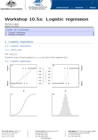
Logistic regression What if y i ∈ { 0, 1 } instead of continuous real value? Disclaimer Even though logistic regression carries regression in its name, it is specifically designed for classification Binary classification Now, datasets are of the form { ( x 1 , 1 ) , ( x 2 , 0 ) , .. } . In this case, linear regression will not do a good job in classifying examples as positive ( y i = 1), or negative ( y i = 0).

Logistic regression Hypothesis space ◮ h a , b ( x ) = g ( � n j = 1 a j x j + b ) = g ( ax + b ) ◮ g ( z ) = 1 1 + e − z is sigmoid function (a.k.a. logistic function) ◮ 0 � g ( z ) � 1, for all z ∈ R z → − ∞ g ( z ) = 0 and lim z → + ∞ g ( z ) = 1 lim ◮ ◮ g ( z ) � 0.5 iff z � 0 ◮ Given example x ◮ predict positive iff h a , b ( x ) � 0.5 iff g ( ax + b ) � 0.5 iff xa + b � 0