A First Supervised Learning Problem How do you measure the biomass - PDF document

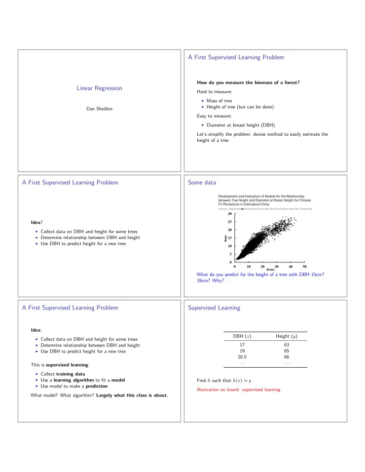
A First Supervised Learning Problem How do you measure the biomass of a forest? Linear Regression Hard to measure: ◮ Mass of tree ◮ Height of tree (but can be done) Dan Sheldon Easy to measure: ◮ Diameter at breast height (DBH) Let’s simplify the problem: devise method to easily estimate the height of a tree A First Supervised Learning Problem Some data Idea ? ◮ Collect data on DBH and height for some trees ◮ Determine relationship between DBH and height ◮ Use DBH to predict height for a new tree What do you predict for the height of a tree with DBH 15cm? 35cm? Why? A First Supervised Learning Problem Supervised Learning Idea : DBH ( x ) Height ( y ) ◮ Collect data on DBH and height for some trees ◮ Determine relationship between DBH and height 17 63 ◮ Use DBH to predict height for a new tree 19 65 20.5 66 · · · · · · This is supervised learning : ◮ Collect training data ◮ Use a learning algorithm to fit a model Find h such that h ( x ) ≈ y ◮ Use model to make a prediction Illustration on board: supervised learning What model? What algorithm? Largely what this class is about.

Supervised Learning: Notation and Terminology Linear Regression in One Variable ◮ Observe m “training examples” of form ( x ( i ) , y ( i ) ) First example of supervised learning. Assume hypothesis is a linear function: ◮ x ( i ) : features / input / what we observe / DBH ◮ y ( i ) : target / output / what we want to predict / height ◮ Training set { ( x (1) , y (1) ) , . . . , ( x ( m ) , y ( m ) ) } h θ ( x ) = θ 0 + θ 1 x ◮ Find function (“hypothesis”) h such that h ( x ) ≈ y ◮ θ 0 : intercept, θ 1 : slope ◮ h ( x ( i ) ) ≈ y ( i ) – good fit on training data ◮ “parameters” or “weights” ◮ Generalize well to new x values How to find “best” θ 0 , θ 1 ? Illustration: hypotheses. Variations: type of x , y , h Finding the best hypothesis Squared Error Cost Function Simplification : “slope-only” model h θ ( x ) = θ 1 x The “squared error” cost function is: ◮ We only need to find θ 1 m J ( θ 1 ) = 1 � h θ ( x ( i ) ) − y ( i ) � 2 � Idea : design cost function J ( θ 1 ) to numerically measure the 2 i =1 quality of hypothesis h θ ( x ) ◮ E.g., θ 1 = 3 : Exercise: which cost functions below make sense? (3 x − y ) 2 / 2 x y 1. A only A. J ( θ 1 ) = � m � h θ ( x ( i ) ) − y ( i ) � (51 − 63) 2 = 144 / 2 17 63 i =1 2. B only (57 − 65) 2 = 64 / 2 19 65 h θ ( x ( i ) ) − y ( i ) � 2 B. J ( θ 1 ) = � m 3. C only � (61 . 5 − 65) 2 = 12 . 25 / 2 i =1 20.5 66 4. B and C C. J ( θ 1 ) = � m � h θ ( x ( i ) ) − y ( i ) � � i =1 � 5. A, B, and C J (3) = (144 + 64 + 12 . 25) / 2 = 220 . 25 / 2 Answer. 4 Our First Algorithm Our First Algorithm In Action We can use calculus to find the hypothesis of minimum cost. Set the derivative of J to zero and solve for θ 1 . For this example: 80 J ( θ 1 ) = 1 � (17 · θ 1 − 63) 2 + (19 · θ 1 − 65) 2 + (20 . 5 · θ 1 − 66) 2 � Height (in.) 70 2 = 535 . 125 · θ 2 1 − 3659 · θ 1 + 6275 60 d 0 = J ( θ 1 ) = 1070 . 25 · θ 1 − 3659 dθ 1 50 16 18 20 22 24 3659 Knee height (in.) θ 1 = 1070 . 25 = 3 . 4188 (See http://www.wolframalpha.com)

The General Algorithm Two Problems Remain In general, we don’t want to plug numbers into J ( θ 1 ) and solve a calculus problem every time . Problem one: we only fit the slope. What if θ 0 � = 0 ? Instead, we can solve for θ 1 in terms of x ( i ) and y ( i ) . Problem two: we will need a better optimization algorithm than d “Set dθ J ( θ ) = 0 and solve for θ .” The general problem: find θ 1 to minimize ◮ Wiggly functions ◮ Equation(s) may be non-linear, hard to solve m J ( θ 1 ) = 1 ( θ 1 x ( i ) − y ( i ) ) 2 � 2 Exercise: ideas for problem one? i =1 You will solve this in HW1. Solution to Problem One Functions of multiple variables! Here is an example cost function: Design a cost function that takes two parameters: m J ( θ 0 , θ 1 ) = 1 2 ( θ 0 + 17 · θ 1 − 63) 2 + 1 J ( θ 0 , θ 1 ) = 1 2 ( θ 0 + 19 · θ 1 − 65) 2 � h θ ( x ( i ) ) − y ( i ) � 2 � 2 2 ( θ 0 + 20 . 5 · θ 1 − 66) 2 + 1 2 ( θ 0 + 18 . 9 · θ 1 − 62 . 9) 2 + . . . + 1 i =1 m = 1 � θ 0 + θ 1 x ( i ) − y ( i ) � 2 � 2 Gain intuition on http://www.wolframalpha.com i =1 ◮ Surface plot Find θ 0 , θ 1 to minimize J ( θ 0 , θ 1 ) ◮ Contour plot Solution to Problem Two: Gradient Descent Gradient Descent To minimize a function J ( θ 0 , θ 1 ) of two variables ◮ Intialize θ 0 , θ 1 arbitrarily ◮ Gradient descent is a general purpose optimization algorithm. A “workhorse” of ML. ◮ Repeat until convergence ◮ Idea: repeatedly take steps in steepest downhill direction, with θ 0 := θ 0 − α ∂ step length proportional to “slope” J ( θ 0 , θ 1 ) ∂θ 0 ◮ Illustration: contour plot and pictorial definition of gradient θ 1 := θ 1 − α ∂ descent J ( θ 0 , θ 1 ) ∂θ 1 ◮ α = step-size or learning rate (not too big)

Partial derivatives Partial derivative intuition ◮ The partial derivative with respect to θ j is denoted ∂ ∂θ j J ( θ 0 , θ 1 ) ∂ Interpretation of partial derivative: ∂θ j J ( θ 0 , θ 1 ) is the rate of ◮ Treat all other variables as constants, then take derivative change along the θ j axis ◮ Example Example: illustrate funciton with elliptical contours ∂u 5 u 2 v 3 = 5 v 3 ∂ ∂ ∂uu 2 ◮ Sign of ∂ ∂θ 0 J ( θ 0 , θ 1 ) ? = 5 v 3 · 2 u ∂ ◮ Sign of ∂θ 1 J ( θ 0 , θ 1 ) ? ◮ Which has larger absolute value? = 10 v 3 u ∂ ∂v 5 u 2 v 3 =?? Gradient Descent The Result in Our Problem 80 ◮ Repeat until convergence Height (in.) 70 θ 0 = θ 0 − α ∂ J ( θ 0 , θ 1 ) ∂θ 0 θ 1 = θ 1 − α ∂ 60 J ( θ 0 , θ 1 ) ∂θ 1 ◮ Issues (explore in HW1) 50 16 18 20 22 24 ◮ Pitfalls Knee height (in.) ◮ How to set step-size α ? ◮ How to diagnose convergence? h θ ( x ) = 39 . 75 + 1 . 25 x Gradient descent intuition Gradient descent for linear regression Algorithm θ j := θ j − α ∂ θ 0 := θ 0 − α ∂ J ( θ 0 , θ 1 ) for j = 0 , 1 J ( θ 0 , θ 1 ) ∂θ j ∂θ 0 θ 1 := θ 1 − α ∂ J ( θ 0 , θ 1 ) Cost function ∂θ 1 m 1 ◮ Why does this move in the direction of steepest descent? � h θ ( x ( i ) ) − y ( i ) � 2 � J ( θ 0 , θ 1 ) = 2 ◮ What would we do if we wanted to maximize J ( θ 0 , θ 1 ) instead? i =1 We need to calculate partial derivatives.

Linear regression partial derivatives Linear regression partial derivatives Let’s first do this with a single training example ( x, y ) : More generally, with many training examples (work this out): m ∂ ∂ ∂ 1 � h θ ( x ( i ) ) − y ( i ) � � � 2 J ( θ 0 , θ 1 ) = J ( θ 0 , θ 1 ) = � h θ ( x ) − y ∂θ 0 ∂θ j ∂θ j 2 i =1 m = 2 · 1 2( h θ ( x ) − y ) · ∂ ∂ � � h θ ( x ( i ) ) − y ( i ) � x ( i ) ( h θ ( x ) − y ) J ( θ 0 , θ 1 ) = ∂θ j ∂θ 1 i =1 � · ∂ � � � h θ ( x ) − y = θ 0 + θ 1 x − y ∂θ j So the algorithm is: m So we get � h θ ( x ( i ) ) − y ( i ) � � θ 0 := θ 0 − α ∂ J ( θ 0 , θ 1 ) = � h θ ( x ) − y � i =1 ∂θ 0 m � � h θ ( x ( i ) ) − y ( i ) � x ( i ) θ 1 := θ 1 − α ∂ J ( θ 0 , θ 1 ) = � h θ ( x ) − y � x i =1 ∂θ 1 Demo: parameter space vs. hypotheses Summary ◮ What to know ◮ Supervised learning setup ◮ Cost function ◮ Convert a learning problem to an optimization problem Show gradient descent demo ◮ Squared error ◮ Gradient descent ◮ Next time ◮ More on gradient descent ◮ Linear algebra review