
SLIDE 1
9/23/2011 1
- L17. Neural processing in Linear Systems 2:
Spatial Filtering
- C. D. Hopkins
- Sept. 23, 2011
Crab cam (Barlow et al., 2001)
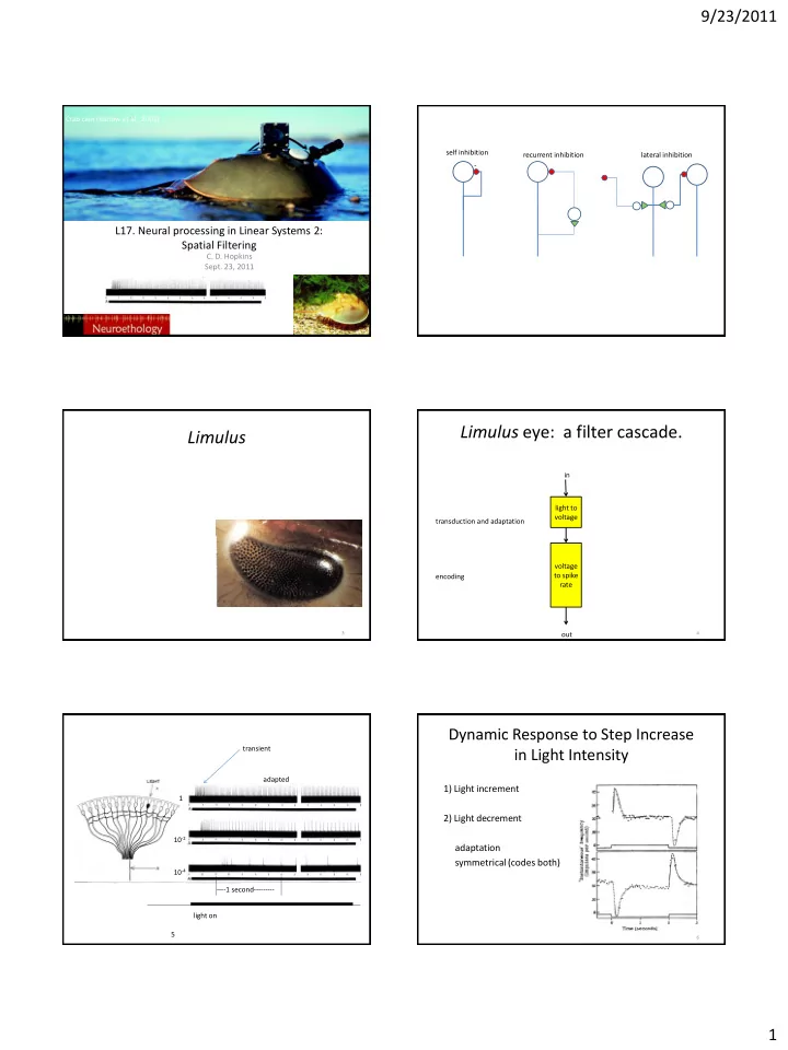
- self inhibition
recurrent inhibition lateral inhibition
3
Limulus
4
Limulus eye: a filter cascade.
transduction and adaptation encoding in
- ut
light to voltage voltage to spike rate 5 light on 1 10-2 10-4
- ---1 second---------
transient adapted
6
Dynamic Response to Step Increase in Light Intensity
1) Light increment 2) Light decrement adaptation symmetrical (codes both)