Lessons from three decades of experiments on household survey - - PDF document

6/4/2018 1

Lessons from three decades of experiments on household survey methods in developing countries

John Gibson, University of Waikato

ADEW, ANU, June 7, 2018

Outline

• Some context

– Survey measurement task gets harder rather than easier as countries escape mass poverty

 opportune time to update survey designs

• Three lessons

– Estimates are sensitive to design variation – Errors are mean‐reverting – Autocorrelations are low

• What we still don’t know

6/4/2018 2

Context:

Data for studying poverty and hunger

• Household consumption (adjusted for demographics)

is the main welfare indicator for poverty and inequality analysis in developing countries

– Considered more reliable than surveyed income and is a closer proxy to permanent income or money metric utility – Available from Household Budget Surveys, Income and Expenditure Surveys, Living Standards Surveys etc

• for almost all countries, and every 2‐5 years for many
• Official (FAO) hunger estimates indirectly use surveys

(to get variance term for spreading national average food availability across population)

– Increasingly, direct measurement of hunger from surveys

Surveys less informative about poverty and hunger than is often realized

• Poverty and hunger estimates are inconsistent across

countries and over time

– Unlike for macro, no general adherence to SNA/BoP manual – unlike for fertility and MCH there is no central agency to dictate survey design everywhere – Matters especially for weak and under‐resourced statistical systems, that are more likely to change from one design to another, with donor‐driven or consultant‐driven change

• More surveys in future ‐‐ World Bank pledged one every 3

years for poorest countries – may not raise understanding

– C.f. only 22 countries having surveys in the first global poverty estimates by Ravallion, Datt & van de Walle (1991)

6/4/2018 3

Surveys less suited to capture distribution of living standards with rising affluence

• poverty becomes harder to measure

– Sociological/compositional effect – Statistical effect

• Sensitivity of poverty to inequality rises, while sensitivity

to growth falls

– Designs that may once have worked for means/totals but do a poor job of measuring dispersion and inequality will increasingly mis‐measure poverty

– Data errors become more important as we focus on the distribution amongst the poor and hungry – People are less compliant and harder to survey

At mass poverty point, CDF almost linear so inequality makes little difference

6/4/2018 4

After escape, poverty line cuts curved part of the CDF so inequality matters

More inequality sensitivity as escape mass poverty

(evidence from Vietnam 2002‐10)

0.0 1.0 2.0 3.0 4.0 5.0 6.0 10 20 30 40 2002 2004 2006 2008 2010 Values derived from elasticities Poverty Rate Head Count Poverty Rate (LHS) Inequality elasticity relative to growth elasticity (RHS) % growth to reduce head count by one point (RHS)

6/4/2018 5

Greater inequality sensitivity also means we need cleaner data

• surveys often have implausible records

– E.g. implied daily per capita calorie availability outside interval

• f, say, 800 ‐ 8,000 (≈ 2000 cal anchors poverty line)

– Due to failure of survey design and/or interview teams to track all flows of incoming and outgoing food ingredients, meals, and/or of people – Measurement errors for households the survey suggests are far below the poverty line have much larger effect on poverty statistics for any distributional‐sensitive measure than is the effect of error for households nearer to the poverty line

• As escape mass poverty, attention often shifts from the

headcount to the distributional‐sensitive measures

Weight placed on measurement error for poor individuals at different values of consumption relative to individual at 90% of the poverty line

Poverty gap index Watts Index and Exit Time Squared poverty gap (FGT‐2) Cubed poverty gap (FGT‐3)

6/4/2018 6

Several types of income elastic consumption are hard to survey

• rising affluence sees new forms of consumption

– Temporally consistent aggregate, reflecting consumption pattern in Vietnam in 1992, was just 78% of the 2010 budget

• housing becomes the largest item in the budget

– Survey measurement of housing services in poor countries is usually very crude, and sometimes dropped from analyses – Or assumed to be fixed ratio to other budget shares given difficulty of measuring this service flow

• E.g. poverty measurement in Vietnam from 1992‐2008 treated

housing as 6% share of total budget

• Once relaxed, housing was 27% share of richest quintile, 8% for

poorest so inequality had been badly mis‐measured

Spatial price variation poorly captured  nominal inequality measures wrong

• Balassa‐Samuelson effect

within‐country

– Housing prices should be higher in richer areas – Nominal inequality will overstate real inequality – Need good spatial price data for deflation but most poor countries have no spatial price surveys – Matters especially if land market emerging from central planning that limited spatial price differences – E.g. China inequality overstated 35%

0.01 0.02 0.03 0.04 0.05 0.06 0.07 0.08 0.09

Real Nominal

Theil Index –

Province‐level, accounting just for spatial price differences for housing 35% bias

6/4/2018 7

Surveys poorly suited to changing diets

• Income elastic food consumption (meals out, more

diverse ingredients) increasingly missed by surveys

– Average food recall list amongst 100 surveys from low/middle income countries has 110 groups

• 14 are various types of cereal ingredients
• Just 3 are categories of meals out of the home

– Meals spending long since exceeded cereal ingredients

• Rice in Vietnam went from one‐third in 1998 to one‐eighth in 2012

while meals out went from 10% to 24% of total food spending

– Common pot reporting unsuited to rapidly urbanizing poor

• Household‐level diary has 29% lower food consumption in urban

Tanzania than a personal diary; in rural areas (where common pot still plausible) the type of diary doesn’t matter

Surveys focus on ingredients yet these matter less

0.05 0.15 0.25 0.35 1998 2000 2002 2004 2006 2008 2010 2012 Share of Total Food Expenditure

Vietnam

Eating Out/Total Food Rice/Total Food

6/4/2018 8

Sociological effect that makes survey measurement harder

• Composition of the poor changes as countries

escape mass poverty

– Poor become less like those who measure them – E.g. ethnic minorities

• Vietnam 1993: with mass poverty, 4 of 5 poor are from

majority group; by 2010 half the poor are minorities

• Different consumption patterns and locations

– Make it harder for general purpose surveys to capture the living standards of the left‐behind poor

• Higher fertility self‐sustains this entrenched poverty

– E.g. India ST/SC fertility 20% above all‐group rate; likewise, higher fertility of poor minority groups in China

Changing composition as escape mass poverty

(evidence from Vietnam 1993‐2010)

6/4/2018 9

Lesson I: Poverty, Hunger, and Inequality Estimates are Sensitive to Survey Design Variation

Based on:

Gibson (2016) “Poverty Measurement: We Know Less Than Policy Makers Realize” Asia & the Pacific Policy Studies 3(3): 430‐442 Beegle, deWeerdt, Friedman & Gibson (2012) “Methods of Household Consumption Measurement through Surveys: Experimental Results from Tanzania” Journal of Development Economics 98(1): 19–33. DeWeerdt, Beegle, Friedman & Gibson (2016) “The Challenge of Measuring Hunger Through Survey” Economic Development and Cultural Change 64(4): 727‐758

18

Some early examples of sensitivity to design variation

 Papua New Guinea: Diaries result in 26% more food

consumption and much lower apparent poverty

 El Salvador: Long recall list results in 31% more

consumption than shorter aggregated list

 Indonesia: Long recall yields 20% more consumption

but no re‐ranking of households

 Ghana: For every day added to recall period, total

purchases fall by 2.9%, plateau at 20‐25% lower

 Russia: Individual diaries gave 6‐11% higher

expenditure than a household diary

6/4/2018 10

Diary‐Recall Sensitivity:

Port Moresby, 1996 PNG HS

20 40 60 80 100 5 6 7 8 9 10

% of population log per capita expenditure

Recall Diary

Poverty line from recall survey

Most convincing evidence is from SHWALITA

20

Module Consumption measurement 1 Long list (58 items) 14 day 2 Long list (58 items) 7 day 3 Subset list (17 items) 7 day 4 Collapsed list (11 items) 7 day 5 Long list (58 items) “Usual 12 month” 6 HH diary with frequent visits 7 HH diary with infrequent visits (by literacy status) 8 Personal diary with daily visits  We randomly assigned (within-village) across Tanzania

8 different consumption modules 500 households each

 Including 1 resource intensive benchmark “Long list”: LSMS has 75 food items on average Approach in the LSMS blue book. Benchmark: not feasible in usual field conditions. 10x as expensive Scaled up

6/4/2018 11

Relative differences between modules

(with or without controls makes no difference) Dependent variable: log per capita consumption

Personal diary omitted Ln total ln food ln non-food, frequent (recall or diary) ln non-food, non-frequent (all recall)

• 1. Recall: Long, 14 day
• 0.161***
• 0.167***
• 0.104
• 0.105*

(0.037) (0.037) (0.067) (0.060)

• 2. Recall: Long, 7 day
• 0.039
• 0.017
• 0.134**
• 0.096

(0.037) (0.037) (0.067) (0.060)

• 3. Recall: Subset, 7 day
• 0.071*
• 0.079**
• 0.112*
• 0.090

(0.037) (0.037) (0.067) (0.060)

• 4. Recall: Collapse, 7 day
• 0.283***
• 0.332***
• 0.104
• 0.138**

(0.037) (0.037) (0.067) (0.060)

• 5. Recall: Long usual 12 month
• 0.207***
• 0.268***

0.023

• 0.013

(0.037) (0.037) (0.067) (0.060)

• 6. Diary: HH, frequent
• 0.173***
• 0.196***
• 0.279***
• 0.046

(0.037) (0.037) (0.067) (0.060)

• 7. Diary: HH, infrequent
• 0.136***
• 0.129***
• 0.244***
• 0.105*

(0.037) (0.037) (0.067) (0.060) Number of households 4,025 4,025 3,942 4,016

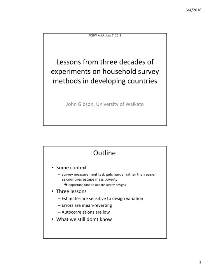
Impact of survey module on poverty

(Headcount poverty rate at $1.25/day line)

10 20 30 40 50 60 70 Long list, 14 day Long list, 7day Subset list, 7d Usual month Diary, HH freq Diary, HH infreq Diary, Indiv

6/4/2018 12

Impact of survey module on poverty

(Poverty Gap Index at $1.25/day poverty line)

5 10 15 20 25 30 35 Long list, 14 day Long list, 7day Subset list, 7d Usual month Diary, HH freq Diary, HH infreq Diary, Indiv

Impact of survey module on poverty

(Squared Poverty Gap Index at $1.25/day poverty line)

2 4 6 8 10 12 14 16 18 Long list, 14 day Long list, 7day Subset list, 7d Usual month Diary, HH freq Diary, HH infreq Diary, Indiv

6/4/2018 13

Average calorie availability

(Kcal per person per day)

500 1000 1500 2000 2500 3000 Long list, 14 day Long list, 7day Subset list, 7d Usual month Diary, HH freq Diary, HH infreq Diary, Indiv

Apparent hunger rate as survey method varies

(% of people in households with energy availability below requirements)

10 20 30 40 50 60 70 Long list, 14 day Long list, 7day Subset list, 7day Usual month Diary, HH freq Diary, HH infreq Individual Diary

6/4/2018 14

Sensitivity to design variation greater for hunger than for poverty

• little scope for design variation for non‐food spending

so the survey modules for these are more standardized

– 6‐month or 12‐month recall typically used – Thus, total value of consumption is (food‐share) weighted average

• f data from standardized and non‐standardized modules

– But calories and hunger depend entirely on the food modules that are the least standardized across surveys

• Hunger estimates are more vulnerable to some key

non‐sampling errors such as consuming food stocks

– Foods that are stocked are low‐value, calorie‐dense foods – Error in measuring consumption from stocks affects $$ much less than it affects calories

False economies from shorter lists

• little time saved by

shortening the recall list by collapsing to major headings or using subsets

• Asking about

“usual” month, as was used in several LSMS, and was recommended to get a more typical measure of living standards, almost doubles the time

10 20 30 40 50 60 70 80

Long list, 14 day Long list, 7 day Subset list, 7 day Collapsed list, 7 day Long list, usual month

minutes to complete food recall in the Tanzania experiment

6/4/2018 15

Why this sensitivity to survey design variation matters

• Impairs cross‐country comparability
• Impairs within‐country monitoring

– Trends are unreliable when survey design changes

• especially in statistically weak countries beholden to

the survey preferences of donors or consultants

– Errors that underlie the sensitivity to different methods will affect different types of households even with nominally the same method

• E.g. household‐level diary works differently in urban

versus rural area

Lesson II: Errors are Mean‐Reverting

Based on: Gibson, Beegle, De Weerdt & Friedman (2015) “What does Variation in Survey Design Reveal about the Nature of Measurement Errors in Household Consumption?” Oxford Bulletin of Economics and Statistics 77(3): 466‐474. Gibson and Kim (2007) “Measurement Error in Recall Surveys and the Relationship Between Household Size and Food Demand” American Journal of Agricultural Economics 89(2): 473‐489.

6/4/2018 16

Why mean‐reversion matters

• Sensitivity to different survey design not easily

fixed with simple adjustment factors

– Errors are related to true values so any correction factor to adjust between survey designs would need to be household‐specific

• Usual mitigation treatment for measurement

error (IV) is unlikely to work

• Relationships may be biased up or down

– E.g. inverse‐size productivity relationship

Comforting, unrealistic, assumptions about measurement error

• Standard assumption is that measurement error

is just white noise added to the true value

– Shown by the reliability ratio for a variable – Mis‐measured consumption as a left‐hand side variable causes no bias – Mis‐measured consumption on right‐hand side has an OLS coefficient that is attenuated in proportion to the reliability ratio

6/4/2018 17

More realistic assumptions: error‐ridden variable on the left

• True model is:
• Observed variable, y* related to true y, by:
• Restrictions for standard assumptions are that:
• with mean‐reverting error,

we get: y x u     

*

y y v     

, ) , cov( ) , cov( ) , cov( ) (     v u v x v y v E 1 ,    

, 1   

*

*

cov( , ) cov( , ) var( ) var( )

y x

y x x u v x x x           

More realistic assumptions: error‐ridden variable on the right

• True model is:
• Observed variable, x* related to true x, by:
• Estimator of the response coefficient is:
• With strong mean‐reversion,  is close to zero and if

denominator < numerator, expands, not attenuates

y x u     

*

x x v     

*

* * 2 * * * 2 2 2

cov( , ) cov( , ) var( ) var( )

x yx x v

x v u x y x x x                     

6/4/2018 18

Implications

• Bias in slopes (e.g. treatment effects estimator)

if consumption is the outcome measure

• Coefficient on consumption on the right‐hand

side (e.g. as a proxy for permanent income or growth effects) could be biased away from zero, unlike for classical error

– No longer certain that our estimates are a lower bound to the true effect

• IV is inconsistent for mean‐reverting errors (and

reverse‐regression bounds typically too wide)

Evidence for mean‐reverting errors

• Pradhan (1999) based on SUSENAS short (core)

and long (module) consumption recall

• 1% increase in average consumption increases the

fraction by which consumption is underestimated by about 0.4 percentage points

• SHWALITA random assignment to one of eight

consumption modules

• Balanced within villages so compare village‐level average

consumption estimates from each module with the benchmark

• Gives direct estimates of 

to test for mean‐reversion

6/4/2018 19

Mean reversion parameter () using SHWALITA village means

0.1 0.2 0.3 0.4 0.5 0.6 0.7 0.8 0.9 1 HH diary, infrequent HH Diary, frequent Long list, usual month Collapsed, 7 day Subset list, 7 day Long list, 7 day Long list, 14 day

Assumed value under standard assumptions

Across SHWALITA survey clusters (7‐day recall)

‐2.0 ‐1.5 ‐1.0 ‐0.5 0.0 0.5 1.0 1.5 2.0

13 14 15 16

Proportionate error (7‐day recall – benchmark)

ln(EA mean consumption from benchmark personal diary)

6/4/2018 20

Doubly‐mean‐reverting errors

• Abay, Abate, Barrett & Bernard (2018) consider

mean‐reverting errors on left‐ and right‐hand side at the same time

– Errors in measuring grain production and in measuring plot size (compass & rope, and GPS measures increasingly used to show mean‐reverting errors in self‐reported plot size)

• Data with no errors on left‐ or right‐hand side show

no inverse‐size productivity relationship

• Errors in both give significant negative elasticity of

productivity with respect to plot size of ‐0.2

– Correcting just one error (either plot size or production) gives even more biased size‐productivity elasticity of ‐0.6

Lesson III: Autocorrelations are Low

Based on: Gibson (2018) “Measuring Chronic Hunger from Diet Snapshots” Economic Development and Cultural Change, forthcoming Gibson and Alimi (2018) “Measuring Poverty with Noisy and Corrected Estimates of Annual Consumption: Evidence from Nigeria” Gibson, Huang & Rozelle (2003) “Improving Estimates of Inequality and Poverty from Urban China's Household Income and Expenditure Survey” Review of Income and Wealth 49(1): 53‐68 Gibson (2001) “Measuring Chronic Poverty Without a Panel” Journal of Development Economics 65(2): 243‐266.

6/4/2018 21

Poverty measurements usually assume autocorrelation in consumption is 1

• Surveys use short reference periods (“snapshots”) for

most components of household consumption

• E.g. weekly, fortnightly or monthly for food

– Assumed easier for respondents to recall over short periods – Asking respondents to report for longer periods increases risk of non‐compliance/fatigue

• See evidence from PNG income and expenditure diaries

– FAO/World Bank now recommend one week food recall

• Poverty/hunger could be defined in weekly terms but

not what policy makers want (e.g. FAO annual hunger)  Naïve extrapolation is used to annualize (weekly  52)

41

Diary Fatigue: 2009/10 PNG HIES

42

3 4 5 6 7 8 9 10 5 10 15 20 25 30 35 40 1 2 3 4 5 6 7 8 9 10 11 12 13 14 Average value per transaction (Kina) Number ('000s), Sum of log value (K'000s) Diary‐Keeping Day Number (LHS) Value (LHS) Average Value (RHS)

6/4/2018 22

Problem with naïve extrapolation

• Measuring poverty and hunger (SDG 1 and 2) involves the

lower tail of distributions

 Need reliable measures of variances as well as means/totals

• Naïve extrapolation of snapshots can give reasonable

estimate of annual means/totals if sample is staggered

• ver the months in the year
• But if autocorrelations < 1, variance is greatly overstated
• Problem is that many shocks occurring in reference period

are subsequently reversed outside the reference period

– Adds intra‐household component to inter‐household variance – Inequality overstated (and poverty, if z is below the mode)

43

Short reference period surveys overstate variances

(and poverty or hunger – for thresholds below the mode)

6/4/2018 23

Why autocorrelations matter

45

• key parameters for correctly annualizing from,

say, monthly reference periods, are correlations between consumption estimates for the same households in all pairs of months in the year

– Inter‐household variance of annual consumption relies on summing the square of each household’s deviation from the all‐households annual mean – annual deviations can be written as a sum of monthly deviations

• monthly deviations are components of the Pearson

product‐moment correlation for the same household’s consumption between any two months of the year

For variances, annual  (monthly12)

46

• Annual mean from monthly as: = 12
• Annual variance of household consumption can

be written as:

– rt,t’ is the correlation between same households value of consumption in months t and t’

• i.e., autocorrelation in consumption

– t is standard deviation across all households in month t







12 1 ' , ' ' ,

) (

t t t t t t a

r x V  

6/4/2018 24

Variances and correlations, continued

47

• If dispersion across households does not vary

from month to month,* we can simplify to:

– V(xm) is variance in the value of monthly consumption, across all i households and t months in the year – ̅ is the average correlation between the same household’s consumption in all pairs of months in the year

*this is unrealistic, e.g. higher variance post‐harvest, but seems to make little difference, empirically

 

) ( 132 12 ) (

xm

a

V r x V   

Overstatement of annual variances depends on ̅

48

• Naïve extrapolation, by multiplying monthly

consumption by 12 gives: = 144

– assumes ̅ 1 (i.e., there is no reshuffling in the monthly ranking of households) – Shocks in the survey reference period cause a deviation from the all‐household, all‐month mean, and naïve extrapolation locks them in as if they happen in each and every month of the year

6/4/2018 25

Variance of short‐period (or naively annualized) relative to annual variance

49 Relax equi-dispersion assumption; let SD be 30% higher in 4 month post-harvest

What do we know about intra‐year autocorrelations?

• Not much
• Researchers and survey agencies have over‐invested in

inter‐year panels and under‐invested in intra‐year panels

– World Bank metadata survey on design of food modules for surveys in 100 low‐ and middle‐income countries has only two surveys with intra‐year panel component

• Not due to lack of $$ for revisiting households

– Diary‐keeping surveys (40% of World Bank sample) have median of four revisits for diary checking, but all in short succession, like five visits in two weeks, so uninformative about ̅ – Ghana LSMS had 11 visits in one month (yet monotonic fall in data quality with each visit – Schündeln, OBES 2018)

50

6/4/2018 26

From limited evidence, correlations for consumption or expenditures are low

51

Setting and welfare indictor

Product‐ moment correlatn Overstatement in variance with naïve extrapoln

PNG – expenditure per adult equivalent 0.6 60% Urban China – household expenditures 0.2 270% Nigeria – value of food consumption 0.4 140% Tonga – household expenditures 0.2 270% Vanuatu – household expenditures 0.4 140%

• Except China, all from single revisit, approximately 6 months

after first observation on consumption

• Mostly for small samples with n<500

New evidence from Myanmar

52

• 2009/10 IHLCA surveys each household’s consumption

twice within the year, in Dec/Jan and again in May

– Large sample (N=18,300)

• detailed record of foods consumed in prior month, using a recall for

228 food and drink groups

• Based on consumption rather than acquisitions and uses local units

to improve recall accuracy

• Includes quantities and calorie contents for 24 types of food out of

the home – much better than typical household surveys

• Results here focus on calories, which should have even

higher autocorrelation than for total consumption

• Households buffer their food budget, and can adjust on

quality margin to preserve food quantity/calorie intakes

6/4/2018 27

Low autocorrelation in calories

53

• Correlation in per capita

calories for same households in two different months is just 0.45

• Evidently not a lot of calorie

smoothing

• Lower for urban than rural
• Volatility comes both from

total calories but also from household size

– Thus, low autocorrelations due to demographic shocks, plus seasonality and other sources

Myanmar Urban Rural

Per capita calories 0.45 0.38 0.44 Total calories 0.68 0.61 0.68 Household size 0.92 0.89 0.93

Inter-month correlations

(Dec/Jan versus May)

Using ̅ 0.45 to get corrected extrapolation

• f annual calories, and chronic hunger rate

54

• Ideally, average inter‐month correlation would

come from multiple months

– Evidence from urban China is that the correlation is similar using revisits once, twice, or five times

• Single revisit to get ̅ gave corrected extrapolation from monthly

to annual expenditures whose headcount poverty rate was just 0.1% off the benchmark rate

• Benchmark from using yearlong diary data of each household
• At ̅ 0.45, deviations from average monthly p.c. calories

scale up by 8.4 rather than by 12 when annualizing

– Some shocks in reference month would partially reverse

6/4/2018 28

Overstated annual hunger if using monthly data for Myanmar

55

.0002 .0004 .0006 .0008 2000 4000 6000 8000 Daily Calories Monthly (or naive extrap) Annual (corrected extrap)

26% < 2000 cal/d 14% < 2000 cal/d

Similar result when estimating poverty in Nigeria

56

• Nigeria GHS has panel

with post‐planting and post‐harvest rounds

– Mix of weekly and monthly recall – use intra‐year correlation to correct extrapolation to annual consumption

• Headcount poverty rate

almost halved in rural areas and has one‐third its naïve value in urban areas

5 10 15 20 25 30 35 40 45 50

Rural Urban Headcount Poverty Rate

Naïve Corrected

6/4/2018 29

Implications

57

• Inter‐month volatility means snapshots will overstate

annual dispersion

– For chronic hunger or poverty snapshot surveys overstate – SDG zero targets; presumably for chronic not transient

• We would learn more by redeploying some survey

resources into revisits ca. six months after first visit than from series of short adjacent revisits

– Similar point made in “more T in experiments”

• Imperfect smoothing just as apparent in urban areas,

and also comes from demographics (household size) so more than just seasonality

– more focus should go on transitory hunger, which FAO ignore

What we don’t know about autocorrelations

• Is single revisit sufficient? Do autocorrelations decay?

– Only have urban China results to rely on here – Multiple revisits would also inform about measurement error

• With 3‐wave panel can use Heise (1969) approach, albeit with

restrictive assumptions (AR(1) for consumption, stable errors)

• Are fluctuations from snapshot surveys just noise or

do they have welfare significance?

– Using the intra‐year correlation to correct extrapolation gives one way to decompose into chronic and transient poverty or chronic and transient hunger, using the components approach to welfare fluctuations

58

6/4/2018 30

What we don’t know more generally

59

• Anthropologists might help us understand how

consumers view food

– Is it primarily as ingredients, which our surveys emphasize – Are there nutritious items that people don’t view as foods?

• Psychologists and lab experimenters might help us

understand how respondents actually answer questions

– Enumeration versus estimation strategies

• Surveys are never explicit on whether the goal is to get respondents

to count/recall/list each occurrence, or instead to give an accurate rule‐of‐thumb estimate

• Respondents clearly switch between these strategies as recall

period lengthens, frequency of events increases and so on, but we have no understanding of when/how this switch occurs

Conclusions

• more surveys does not necessarily mean better

measurement of poverty and hunger

– Especially for the left‐behind poor

• We could better measure poverty and hunger if

surveys:

– Settled on harmonized designs, e.g. 7‐day food recall – Redeployed interview resources so the same households are observed 2‐3 times within the year (in non‐adjacent periods)

• Our analyses would be more robust if we factored in

the likelihood of mean‐reverting errors

6/4/2018 31

Acknowledgements

• Collaborators

– Kathleen Beegle – World Bank – Joachim de Weerdt – EDI and University of Antwerp – Jed Friedman – World Bank – Bonggeun Kim – Seoul National University – Scott Rozelle – Stanford University

• Funders and supporters

– World Bank – Food and Agriculture Organization of the UN

Thank You