Lehmann & Romano, TSH Ch. 3 Setup: define a test function ( y ) - PowerPoint PPT Presentation

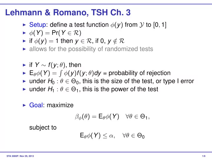
Lehmann & Romano, TSH Ch. 3 ◮ Setup: define a test function φ ( y ) from Y to [ 0 , 1 ] ◮ φ ( Y ) = Pr ( Y ∈ R ) ◮ if φ ( y ) = 1 then y ∈ R , if 0, y / ∈ R ◮ allows for the possibility of randomized tests ◮ if Y ∼ f ( y ; θ ) , then ◮ E θ φ ( Y ) = � φ ( y ) f ( y ; θ ) dy = probability of rejection ◮ under H 0 : θ ∈ Θ 0 , this is the size of the test, or type I error ◮ under H 1 : θ ∈ Θ 1 , this is the power of the test ◮ Goal: maximize β φ ( θ ) = E θ φ ( Y ) ∀ θ ∈ Θ 1 , subject to E θ φ ( Y ) ≤ α, ∀ θ ∈ Θ 0 STA 3000F: Nov 29, 2013 1/9

Neyman-Pearson lemma ◮ Suppose Θ 0 is the point θ 0 , and similarly for Θ 1 ◮ Assume the existence of densities f 0 and f 1 with respect to the same measure µ 1. Given 0 ≤ α ≤ 1, there exists a test function φ and a constant k such that E 0 φ ( Y ) = α (1) and � 1 when f 1 ( y ) > kf 0 ( y ) , φ ( y ) = (2) f 1 ( y ) < kf 0 ( y ) . 0 when 2. If a test satisfies (1) and (2) for some k , then it is most powerful for testing f 0 against f 1 at level α 3. If φ is most powerful at level α for testing f 0 against f 1 , then for some k it satisfies (2), a.e. µ , and satisfies (1) unless there exists a test of size < α and with power 1. STA 3000F: Nov 29, 2013 2/9

Proof 1. ◮ trivial for α = 0 and α = 1 allow k = ∞ ◮ 1. define α ( c ) = Pr 0 { f 1 ( Y ) > cf 0 ( Y ) } = Pr { f 1 ( Y ) / f ) 0 ( Y ) > c } . ◮ 1 − α ( c ) is a cumulative distribution function ◮ so α ( c ) is non-increasing, right-continuous, α ( −∞ ) = 1 , α ( ∞ ) = 0 ◮ Given 0 < α < 1, let c 0 be such that α ( c 0 ) ≤ α ≤ α ( c − 0 ) ◮  f 1 ( y ) > c 0 f 0 ( y ) 1 when   α − α ( c 0 ) when f 1 ( y ) = c 0 f 0 ( y ) φ ( y ) = α ( c − 0 ) − α ( c 0 )  0 when f 1 ( y ) < c 0 f 0 ( y )  ◮ � f 1 ( Y ) � E 0 φ ( Y ) = Pr 0 + f 0 ( Y ) STA 3000F: Nov 29, 2013 3/9

... proof 2. ◮ Suppose φ is a test satisfying (1) and (2), and that φ ∗ is another test with E 0 φ ∗ ( Y ) ≤ α . ◮ Denote by S + and S − the sets in Y where φ ( y ) − φ ∗ ( y ) > 0 and < 0. ◮ In S + , φ ( y ) > 0 so f 1 ( y ) ≥ kf 0 ( y ) , and ◮ � � ( φ − φ ∗ )( f 1 − kf 0 ) d µ = S + ∪ S − ( φ − φ ∗ )( f 1 − kf 0 ) d µ ≥ 0 ◮ difference in power: � � ( φ − φ ∗ ) f 1 d µ ≥ k ( φ − φ ∗ ) f 0 d µ ≥ 0 STA 3000F: Nov 29, 2013 4/9

... proof 3. ◮ Let φ ∗ be MP level α , and φ satisfy (1) and (2) ◮ On S + ∪ S − , φ and φ ∗ differ. Let S = S + ∪ S − ∩ { y : f 1 ( y ) � = kf 0 ( y ) } , and assume µ ( S ) > 0 ◮ � � S + ∪ S − ( φ − φ ∗ )( f 1 − kf 0 ) d µ = ( φ − φ ∗ )( f 1 − kf 0 ) d µ > 0 S ◮ implies φ is more powerful than φ ∗ ◮ contradiction, hence µ ( S ) = 0 ◮ if φ ∗ had size < α and power < 1, could add points to rejection region until either E 0 φ ∗ ( Y ) = α or E 1 φ ∗ ( Y ) = 1 ◮ test is unique if { y : f 1 ( y ) = kf 0 ( y ) } has measure 0 STA 3000F: Nov 29, 2013 5/9

Comments ◮ discreteness: e.g. Y ∼ Bin ( n , p ) ◮ MP test has rejection region R determined by { y > d α } ◮ not all values of α attainable: e.g. CH Example 4.9 Y ∼ Poisson ( µ ) ◮ H 0 : µ = 1 , H 1 : µ = µ 1 > 1, MP test Y ≥ d α Table : attained significance levels Pr ( Y > y ; µ = 1 ) Pr ( Y > y ; µ = 1 ) y y 0 1 4 0.0189 1 0.632 5 0.0037 2 0.264 6 0.0006 . . . . 3 0.080 . . ◮ if critical regions are nested , i.e. R α 1 ⊂ R α 2 , α 1 < α 2 , then p obs = inf ( α ; y obs ∈ R α ) ◮ asymmetry: Y ∼ N ( µ, 1 ) , H 0 : µ = 0 , H 1 : µ = 10 , y obs = 3 STA 3000F: Nov 29, 2013 6/9

Bayesian testing see CH Example 10.12 ◮ simple H 0 , simple H 1 : Pr ( H 0 | y ) Pr ( H 1 | y ) = Pr ( H 0 ) f 0 ( y ) Pr ( H 1 ) f 1 ( y ) ◮ similarly, with H 1 , . . . H k potential alternatives Pr ( H 0 | y ) 0 | y ) = Pr ( H 0 ) f 0 ( y ) Pr ( H c Σ j Pr ( H j ) f j ( y ) ◮ sharp null hypothesis: H 0 : θ = θ 0 , H 1 : θ � = θ 0 Pr ( H 0 | y ) π 0 f ( y ; θ 0 ) 0 | y ) = Pr ( H c � ( 1 − π 0 ) π 1 ( θ ) f ( y ; θ ) d θ ◮ nuisance parameters Pr ( H 0 | y ) π 0 π ( λ | h 0 ) f ( y | ψ 0 , λ ) d λ 0 | y ) = Pr ( H c � � ( 1 − π 0 ) π ( ψ, λ | H 1 ) f ( y | ψ, λ ) d ψ d λ STA 3000F: Nov 29, 2013 7/9

... testing ◮ Bayes factor B 10 = Pr ( y | H 1 ) Pr ( y | H 0 ) ◮ typically Pr ( y | h i ) = � f ( y | H i , θ i ) π ( θ i | H i ) d θ i , i = 0 , 1 SM Ch. 11.2 ◮ cannot be computed with improper priors STA 3000F: Nov 29, 2013 8/9

Nature, PNAS, AoS articles by Johnson ◮ developed an ‘objective’ Bayesian test for comparison to p -values ◮ “A p -value of 0.05 or less corresponds to Bayes factors of between 3 and 5, which are consider weak evidence to support a finding” ◮ “He advocates for scientists to use more stringent p -values of 0.005 or less” ◮ see also CH Example 10.12 and SM Example 11.15 ◮ emphasis on point hypotheses drives most of these anomalous results ◮ e.g. Pr ( θ > 0 | y ) STA 3000F: Nov 29, 2013 9/9