Lecture 3: Linear Regression (Part 2) Feb 3rd 2020 Lecturer: Steven - - PDF document

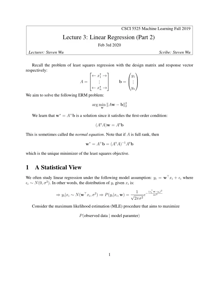
CSCI 5525 Machine Learning Fall 2019

Lecture 3: Linear Regression (Part 2)

Feb 3rd 2020 Lecturer: Steven Wu Scribe: Steven Wu Recall the problem of least squares regression with the design matrix and response vector respectively: A =    ← x⊺

1 →

. . . ← x⊺

n →

   b =    y1 . . . yn    We aim to solve the following ERM problem: arg min

w Aw − b2 2

We learn that w∗ = A+b is a solution since it satisfies the first-order condition: (A⊺A)w = A⊺b This is sometimes called the normal equation. Note that if A is full rank, then w∗ = A+b = (A⊺A)−1A⊺b which is the unique minimizer of the least squares objective.

1 A Statistical View

We often study linear regression under the following model assumption: yi = w⊤xi + ǫi where ǫi ∼ N(0, σ2). In other words, the distribution of yi given xi is: ⇒ yi|xi ∼ N(w⊤xi, σ2) ⇒ P(yi|xi, w) = 1 √ 2πσ2e−

(x⊤ i w−yi)2 2σ2

Consider the maximum likelihood estimation (MLE) procedure that aims to maximize P(observed data | model paramter) 1

In more details: w = argmax

w

P(y1, x1, ..., yn, xn|w) = argmax

w n

• i=1

P(yi, xi|w) (Independence) = argmax

w n

• i=1

P(yi|xi, w)P(xi|w) (Chain rule of probability) = argmax

w n

• i=1

P(yi|xi, w)P(xi) (xi is independent of w) = argmax

w n

• i=1

P(yi|xi, w) (P(xi) does not depend on w) = argmax

w n

• i=1

log [P(yi|xi, w)] (log is a monotonic function) = argmax

w n

• i=1
• log
• 1

√ 2πσ2

• + log
• e−

(x⊤ i w−yi)2 2σ2

• (Plugging in Gaussian distribution)

= argmax

w

− 1 2σ2

n

• i=1

(x⊤

i w − yi)2

(First term is a constant, and log(ez) = z) = argmin

w

1 n

n

• i=1

(x⊤

i w − yi)2

Now consider a similar maximum a posteriori estimation (MAP) with a prior assumption: P(w) = 1 √ 2πτ 2e− w⊤w

2τ2

The MAP estimation instead aims to solve P(model parameter | observed data) 2

w = argmax

w

P(w|y1, x1, ..., yn, xn) = argmax

w

P(y1, x1, ..., yn, xn|w)P(w) P(y1, x1, ..., yn, xn) = argmax

w

P(y1, x1, ..., yn, xn|w)P(w) = argmax

w

n

• i=1

P(yi, xi|w)

• P(w)

= argmax

w

n

• i=1

P(yi|xi, w)P(xi|w)

• P(w)

= argmax

w

n

• i=1

P(yi|xi, w)P(xi)

• P(w)

= argmax

w

n

• i=1

P(yi|xi, w)

• P(w)

= argmax

w n

• i=1

log P(yi|xi, w) + log P(w) = argmin

w

1 2σ2

n

• i=1

(x⊤

i w − yi)2 + 1

2τ 2w⊤w = argmin

w

1 n

n

• i=1

(x⊤

i w − yi)2 + λ||w||2 2

λ =

σ2 nτ 2

This actually corresponds to a regularized ERM problem called ridge regression.

2 Ridge Regression

Now consider following regularized ERM problem called ridge regression: min

w Aw − b2 2 + λw2 2

(1) Now let’s replace A⊺A by (A⊺A + λI) in the ordinary least squares solution and obtain: ˆ w = (A⊺A + λI)−1A⊺b. (2) Again, by first-order condition, we can show that ˆ w is the the solution to (1). Note that the solution is always unique even if A is not full rank (e.g., when n < d). The regularization or penalty term 3

λw2

2 encourages “shorter” solutions w with smaller ℓ2 norm. The paramter λ manages the trade-

• ff between fitting the data to minimize ˆ

R and shrinking the solution to minimize λw2

• 2. Ridge

regression can also be formulated as a constrained optimization problem: min

w Aw − b2 2

such that w ≤ β. Why do we care to make the weights w short or small? Intuively, larger w corresponds to higher model complexity. By bounding the model complexity, we can prevent overfitting—that is the model has small training error, but large test error. However, if we bound the norm of w to aggressively (by setting λ to be very large), then we might run into the problem of underfitting— that is the model has large training error and test error. Lasso regression. Another common regularization is the Lasso regression that uses ℓ1 penalty: arg min

w Aw − b2 2 + λw1

Lasso encourages sparse solutions, and is commonly used when d is much greater than the number

• f observations n. However, it does not admit a closed-form solution.

3 Feature Transformation

We can enrich linear regression models by transforming the features: first transform each feature vector x into φ(x), and then predict by using linear function over the transformed features, that is ˆ f(x) = w⊺φ(x). Consider the following examples of feature transformation:

• for x ∈ R, φ(x) = ln(1 + x)
• for x ∈ {0, 1}d, we can apply boolean functions such as

φ(x) = (x1 ∧ x2) ∨ (x3 ∨ x4)

• for x ∈ Rd, we can also apply polynomial expansion:

φ(x) = (1, x1, . . . , xd, x2

1, . . . , x2 d, x1x2, . . . , xd−1xd)

• for x ∈ R, we can also apply trigonometry expansion:

φ(x) = (1, sin(x), cos(x), sin(2x), cos(2x), . . .) Can we just use complicated linear mapping though? No, we won’t gain anything: w⊺φ(x) is just another linear function of x, when φ is also a linear mapping of x. Feature engineering can get messy, and often requires a lot of domain knowledge. For example, we probably should not use polynomial expansion for periodic data. 4

Figure 1: Examples shown in class. Fitting a linear function versus fitting a degree-3 polynomial. (More details here.)

4 Hyperparameters, Validation Set, and Test Set

The parameter λ in ridge regression and Lasso regression, and the order of polynomials in polyno- mial expansion, and also the paramter k in k-nearest neighbor are often called hyperparamters for the machine learning algorithms, which requires tuning. How do we optimize these parameters? A standard way is to perform the following three-way data splits:

• Training set: learn the predictor ˆ

f (e.g. weight vector w) by “fitting” this dataset.

• Validation set: a set of examples to tune the hyperparameters. We use the loss on this dataset

to find the “best” hyperparameter.

• Test set: we use this data to assess the risk of the final model:

R(f) = E

(X,Y )∼P[ℓ(Y, f(X))]

In the case of squared loss, this is R(f) = E

(X,Y )∼P[(f(X) − Y )2]

In general, we want to predict well on future instances, so the goal is formulated as finding a predictor ˆ f that minimizes the risk (instead of empirical risk on the training set). What if we did not start with a validation set? We can always create a validation set from the training set. One standard method is cross validation. k-fold cross validation We split the training set into k parts or folds of roughly equal size: F1, . . . , Fk. (Typically, k = 5 or 10, but it also depends on the size of your dataset.)

• 1. For j = 1, . . . , k:
• We will train on the union of folds F−j =

j′=j Fj′ and validate on fold Fj

5

• For each value of the tuning parameter θ ∈ {θ1, . . . , θm}, train on F−j to obtain predic-

tor ˆ f −j

θ , and record the loss on the validation set ˆ

Rj( ˆ f −j

θ )).

• 2. For each paramter θ, compute the average loss over all folds

ˆ RCV(θ) = 1 k

k

• j=1

ˆ Rj( ˆ f −j

θ )

Then we will chose the parameter ˆ θ that minimize ˆ RCV(θ). 6