Lecture 21: Bootstrap and Permutation Tests The bootstrap - - PDF document

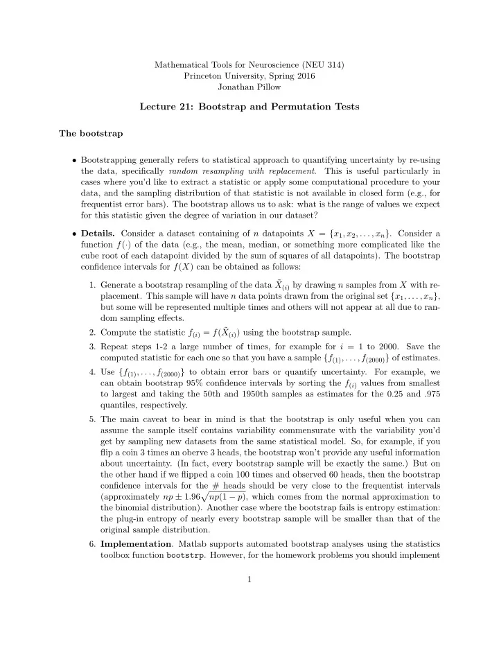
Mathematical Tools for Neuroscience (NEU 314) Princeton University, Spring 2016 Jonathan Pillow

Lecture 21: Bootstrap and Permutation Tests

The bootstrap

• Bootstrapping generally refers to statistical approach to quantifying uncertainty by re-using

the data, specifically random resampling with replacement. This is useful particularly in cases where you’d like to extract a statistic or apply some computational procedure to your data, and the sampling distribution of that statistic is not available in closed form (e.g., for frequentist error bars). The bootstrap allows us to ask: what is the range of values we expect for this statistic given the degree of variation in our dataset?

• Details. Consider a dataset containing of n datapoints X = {x1, x2, . . . , xn}. Consider a

function f(·) of the data (e.g., the mean, median, or something more complicated like the cube root of each datapoint divided by the sum of squares of all datapoints). The bootstrap confidence intervals for f(X) can be obtained as follows:

• 1. Generate a bootstrap resampling of the data ˜

X(i) by drawing n samples from X with re-

• placement. This sample will have n data points drawn from the original set {x1, . . . , xn},

but some will be represented multiple times and others will not appear at all due to ran- dom sampling effects.

• 2. Compute the statistic f(i) = f( ˜

X(i)) using the bootstrap sample.

• 3. Repeat steps 1-2 a large number of times, for example for i = 1 to 2000.

Save the computed statistic for each one so that you have a sample {f(1), . . . , f(2000)} of estimates.

• 4. Use {f(1), . . . , f(2000)} to obtain error bars or quantify uncertainty.

For example, we can obtain bootstrap 95% confidence intervals by sorting the f(i) values from smallest to largest and taking the 50th and 1950th samples as estimates for the 0.25 and .975 quantiles, respectively.

• 5. The main caveat to bear in mind is that the bootstrap is only useful when you can

assume the sample itself contains variability commensurate with the variability you’d get by sampling new datasets from the same statistical model. So, for example, if you flip a coin 3 times an oberve 3 heads, the bootstrap won’t provide any useful information about uncertainty. (In fact, every bootstrap sample will be exactly the same.) But on the other hand if we flipped a coin 100 times and observed 60 heads, then the bootstrap confidence intervals for the # heads should be very close to the frequentist intervals (approximately np ± 1.96

• np(1 − p), which comes from the normal approximation to

the binomial distribution). Another case where the bootstrap fails is entropy estimation: the plug-in entropy of nearly every bootstrap sample will be smaller than that of the

• riginal sample distribution.
• 6. Implementation. Matlab supports automated bootstrap analyses using the statistics

toolbox function bootstrp. However, for the homework problems you should implement 1

the resampling analyses yourself using the function randsample, which returns a random sample from a set (with or without replacement). Permutation Tests

• Permutation-based analyses resemble the bootstrap in that they rely on randomizations of

the observed data. The primary difference is that while bootstrap analyses typically seek to quantify the sampling distribution of some statistic computed from the data, permutation analyses typically seek to quantify the null distribution. That is, they seek to break whatever structure might be preset in a dataset, and quantify the kinds of patterns one expects to see “purely by chance.”

• Details. We will consider permutation tests in the context of regression or classification tasks

in which the data come in pairs {(xi, yi)}, for i = 1, . . . , n. The idea of a permutation analysis is to randomly permute (or “shuffle”) the xi’s with respect to the yi’s so that any statistical relationship between them is lost. If we estimate regression weights or class labels from many repeated randomly permuted datasets, we can use the resulting samples to characterize the null distribution of the weights, that is, the distribution we would expect if there were no statistical relationship between x and y. Note however that there are a wide variety of different kinds of permutation analyses, depend- ing on the null hypothesis of interest. The common thread is that one seeks to permute the data in a way that removes some aspects of the statistical structure while possibly preserving

• thers (e.g., the relationship between the individual entries in the x vectors).
• Implementation. The matlab function randperm, which generates a random permuation of

the integers 1 to n, is handy for permutation analyses. Classes of Machine learning problems Lastly, we discussed a high level view of the kinds of statistical or machine learning problems that we have examined in this class (plus a few that we didn’t).

• One possible division is between supervised and unsupervised problems.
• Supervised problems involve data that come in pairs, (

xi, yi), and the goal is to estimate a mapping from the xi to the labels or “targets” yi in a way that minimizes error.

• 1. Regression. If the y’s are continuous then we refer to the problem as regression. (In

this course, we covered least-squares regression as the most prominent example).

• 2. Classification. If the y’s are discrete, we typically refer to it as classification. Tech-

nically logistic regression can be considered a classification model (the training data consist of y’s that take on binary values 0 and 1), but we can consider it regression since the model produces a continuous probability that an input vector is assigned to 0 or 1. 2

• Unsupervised problems, by contrast, involve datasets without labels, e.g., where the raw

data are a set of vectors {xi}. Prominent unsupervised learning problems include density estimation (estimating the parameters governing the distribution that generated the data)., dimensionality reduction (e.g. PCA), and clustering (e.g., k-means clustering, which we didn’t cover but probably should have!).

• Reinforcement learning is a third kind of machine learning problem (that we didn’t con-

sider at all in this class). Reinforcment learning (RL) can be considered a special kind of supervised learning problem in which the supervision signal is weak and delayed in time. RL problems typically involve choosing actions that affect the probability of future states and future rewards, and the rewards may be sparse and delayed in time relative to the actions that led to them. Example RL problems include training a rat to navigate a maze, or training a computer to beat humans at go. 3