Learning in Bayes Nets Bayes Nets: 1. Parameter Learning/Estimation: - - PowerPoint PPT Presentation

Bayes Nets: Learning Parameters and Structure

Machine Learning 10-701 Anna Goldenberg

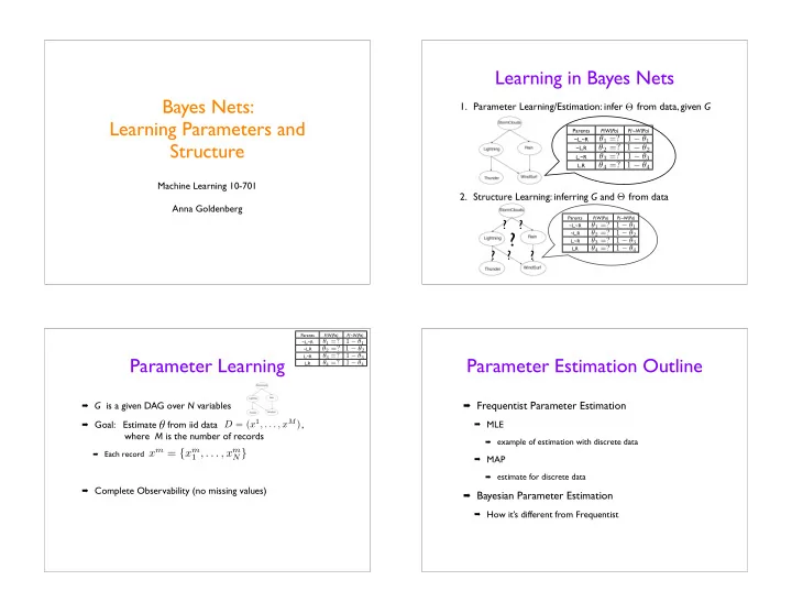
• 1. Parameter Learning/Estimation: infer from data, given G
• 2. Structure Learning: inferring G and from data

Learning in Bayes Nets

Θ

Parents P(W|Pa) P(~W|Pa) ~L,~R

θ1 =? 1 − θ1

~L,R

θ2 =? 1 − θ2

L,~R

θ3 =? 1 − θ3

L,R

θ4 =? 1 − θ4

Θ

? ? ? ? ?

?

Parents P(W|Pa) P(~W|Pa) ~L,~R

θ1 =? 1 − θ1

~L,R

θ2 =? 1 − θ2

L,~R

θ3 =? 1 − θ3

L,R

θ4 =? 1 − θ4

Parameter Learning

G is a given DAG over N variables Goal: Estimate from iid data ,

where M is the number of records

Each record

Complete Observability (no missing values)

θ

D = (x1, . . . , xM)

xm = {xm

1 , . . . , xm N}

Parents P(W|Pa) P(~W|Pa) ~L,~R

θ1 =? 1 − θ1

~L,R

θ2 =? 1 − θ2

L,~R

θ3 =? 1 − θ3

L,R

θ4 =? 1 − θ4

Parameter Estimation Outline

Frequentist Parameter Estimation

MLE

example of estimation with discrete data

MAP

estimate for discrete data

Bayesian Parameter Estimation

How it’s different from Frequentist

Maximum Likelihood Estimator

Likelihood (for iid data): Log likelihood MLE advantages: has nice statistical properties disadvantages: can overfit

ˆ θML = arg max

θ

l(θ; D)

p(D|θ) =

• m
• i

p(xm

i |xm πi, θ)

l(θ; D) = log p(D|θ) =

• m
• i

log p(xm

i |xm πi, θ)

Example: MLE for one variable

Variable X ~ Multinomial with K values (K-sided die) Observe M rolls: 1, 4, K, 2, ... model , (2)

p(X = k) = θk

• k

θk = 1

l(θ; D) =

• m

log

• I(xm = k)θk =
• k
• m

I(xm = k) log(θk) =

• k

Nklog(θk) (1)

Maximizing (1) subject to constraint (2): ˆ θk,ML = Nk M

the fraction of times k occurs

Discrete Bayes Nets

Assume each CPD is represented as a table Loglikelihood: Parameter Estimator:

<=>

Continuous Variables

Example: Gaussian Variables One variable: ML estimates:

ˆ µML =

• m xm

M ˆ σ2ML =

• m(xm − ˆ

µML)2 M

X ∼ N(µ, σ)

Similarly for several Continuous Variables Another option to estimate parameters: Xi ∼ f(Pai, θ)

Maximum A Posteriori estimate (MAP)

MLE is obtained by maximizing loglikelihood sensitive to small sample sizes MAP comes from maximizing posterior prior acts as a smoothing factor

p(θ|D) ∼ p(D|θ)p(θ) = likelihood × prior

Example: MAP for Multinomial

Multinomial likelihood: Dirichlet Prior: Posterior:

MAP

ˆ θMAP

ijk

= Nijk + αijk

• j(Nijk + αijk)

can be thought of as virtual pseudo counts

α

P(D|θ) =

• m
• ijk

θNijk

ijk

P(θ|α) =

• ijk θ(αijk−1)

ijk

Z(α)

P(θ|D, α) ∝

• ijk

θNijk+αijk−1

ijk

Bayesian vs Frequentist

Frequentist:

are unknown constants MLE is a very common frequentist estimator

Bayesian

unknown are random variables estimates differ based on a prior

θ θ

Questions on Parameter Learning?

What if G is not given?

When?

Scientific discovery (protein networks, data mining) Need a good model for compression, prediction...

Structural Learning

Constraint Based

Test independencies Add edges according to the tests

Search and Score

Define a selection criterion that measures goodness of a model Search in the space of all models (or orders)

Mix models (recent)

Test for almost all independencies Search and score according to possible

Constraint Based Learning

Define Conditional Independence Test Ind(Xi;Xj|S)

e.g. ,

G2, conditional entropy, etc.

if Ind(Xi;Xj|S)<p, then independence

Choose p with care! Construct model consistent with the set of independencies

χ2 :

• xi,xj

(Oxi,xj|s − Exi,xj|s)2 Exi,xj|s

Constraint Based Learning

Cons:

Independence tests are less reliable on small samples One incorrect independence test might propagate far (not robust to

noise) Pros:

More global decisions => doesn’t get stuck in local minima as much Works well on sparse nets (small markov blankets, sufficient data)

Score Based Search Outline

Select the highest scoring model! What should the score be? Specialized structures (trees, TANs) Selection operators - how to navigate the space of models?

Theorem: maximizing Bayesian Score for d2 (not a tree) is NP-hard (Chickering, 2002)

Maximum likelihood in Information Theoretic terms

The entropy does not depend on the current model Thus, it’s enough to maximize mutual information! General case:

Same as constraint search!

Special case (trees):

have to consider only all pairs (tree => only one parent): O(N2)

log P(D|θG, G) = M

• i

ˆ I(Xi|PaXi) − M

• i

ˆ H(Xi)

Chow Liu tree algorithm

Compute empirical distribution: Mutual Information: Set as weight per edge between Xi and Xj Find Optimal tree BN by getting the maximum spanning tree

for direction: pick a random node as root direct in BFS order

Tree Augmented Naive Bayes

TAN (Friedman et al, 1997) is an extension of Chow Liu

C X1 X2 X3 XM C X1 X2 X3 XM

Naive Bayes TAN

TAN: Score(TAN):

• i

ˆ I(Xi, C) +

• j

ˆ I(Xj, {PaXj, C})

MI Problem

Doesn’t penalize complexity: I(A,B) I(A,{B,C}) Adding a parent always increases the score! Model will overfit, since the completely connected

graph would be favored

Penalized Likelihood Score

BIC (Bayesian Information Criterion)

, where d is the number of free parameters

AIC (Akaike Information Criterion) BIC penalizes complexity more than AIC

logP(D) ∼ logP(D|ˆ θML) − d 2 log (N) logP(D) ∼ logP(D|ˆ θML) − d

Minimum Description Length

Total number of bits needed to describe data is -log2P(x) Instead - send the model and then residuals:

• L(D,H) = - logP(H) - log P(D|H) = -log P(H|D) + const

The best is the one with the shortest message!

What should the score be?

Consistent : for all G’ I-equivalent to the true G and

all G* not equivalent to G Score(G)=Score(G’) and Score(G*)<Score(G’)

Decomposable : can be locally computed (for efficiency)

Score(G; D) =

• i

FamScore(Xi|PaXi; D)

Example: BIC and AIC are consistent and decomposable

Bayesian Scoring Parameter Prior

Parameter Prior - important for small datasets! Dirichlet Parameters ( from a few slides before ) For each possible family define a prior distribution Can encode it as a Bayes Net (Usually Independent - product of marginals)

Bayesian Scoring Parameter Prior

Bayes Dirichlet equivalent scoring (BDe) : Is consistent (and decomposable)

Theorem: If P(G) assigns the same prior to I-equivalent structures and Parameter prior is Dirichlet then Bayesian score satisfies score equivalence, if and only if prior is of BDe form!

• αXi|P aXi = MP (Xi, Pa(Xi))

Bayesian Scoring Structure Prior

Structure Prior - should satisfy prior modularity Parameter Modularity: if X has the same set of parents

in two different structures, then parameters should be the same.

Typically set to uniform. Can be a function of prior counts:

1 α + 1

Structure search algorithms

Order in known Order is unknown

Search in the space of orderings Search in the space of DAGs Search in the space of equivalence classes

Order is known

Suppose the total ordering is Then for each node Xi can find an optimal set of parents in Choice of parents for Xj doesn’t depend on previous Xi Need to search among all choices (where d is the

maximum number of parents) for the highest local score

Greedy search with known order, aka K2 algorithm is

Order is unknown Search space of orderings

Select an order according to some heuristic Use K2 to learn a BN corresponding to the

• rdering and score it

Maybe do multiple restarts Most recent research: Tessier and Koller (2005)

Order is unknown Search space of DAGs

Typical search operators Add an edge Remove an edge Reverse an edge At most O(n2) steps to get from any graph to any graph Moves are reversible Simplest search is Greedy Hillclimbing Move to proposed new graph if it satisfies constraints

Exploiting Decomposable Score

If the operator for edge (X,Y) is valid, then we need

• nly to look at the families of X and

Y

e.g. for addition operator o

Evaluating costs of moves

Total O(N^2) operators For each operator need to check for acyclicity O(e)

For local moves check acyclicity in amortized O(1) using ancestor matrix

If new graph is acyclic, need to score it (amortized) O(M) K steps to convergence Total time O(K N^2 M) For large M can use AD Trees to compute counts in sub

linear time

Suboptimality

Hillclimbing might get stuck in local maxima Local maxima are common because of equivalent classes Solutions

Random restarts TABU: do not undo up to L latest steps Data perturbation Simulated Annealing (slow!)

Other operators

Optimal Reinsertion (Moore and Wong, 2003)

Start with an arbitrary DAG At every step sever all the edges of a given node Reinsert it optimally

(find best set of parents and children)

Random restart if necessary

Pros: works much faster and is less prone to get stuck in local minima

Searching in space of equivalent classes (GES)

Pros: Space of equivalent classes is smaller Cons: Operators are more complicated

Harder to implement

Empirically shown to have outperformed Greedy

Hillclimbing

Proved to find an optimal BN as M

Constraint+Score Algorithms

Tsamardinos et al, 2005

Find edges via independence tests Find final structures from the pool of edges using hill-

climbing Claims to be faster than most of the algorithms described above!!!

Current problems with Structural Search

• 1. Scalability
• 2. Scalability
• 3. Scalability
• 4. Assumption that data samples are iid

Note: there are special purpose algorithms that scale...

Questions on Structural Learning?