Greedy algorithms Problem. Given a digraph G = ( V , E ) , edge - - PowerPoint PPT Presentation

Greedy algorithms

Shortest paths in weighted graphs Tyler Moore

CS 2123, The University of Tulsa

Some slides created by or adapted from Dr. Kevin Wayne. For more information see http://www.cs.princeton.edu/~wayne/kleinberg-tardos. Some code reused from Python Algorithms by Magnus Lie Hetland.

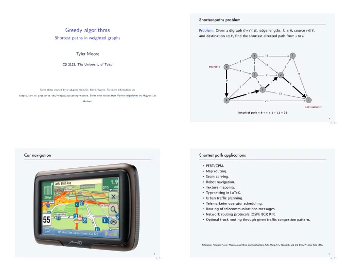
• Problem. Given a digraph G = (V, E), edge lengths ℓ

e ≥ 0, source s ∈ V,

and destination t ∈ V, find the shortest directed path from s to t.

Shortest-paths problem

3

7 1 3 source s 6 8 5 7 5 4 15 3 12 20 13 9 length of path = 9 + 4 + 1 + 11 = 25 destination t 4 5 2 6 9 4 1 11 2 / 21

Car navigation

4

3 / 21

・PERT/CPM. ・Map routing. ・Seam carving. ・Robot navigation. ・Texture mapping. ・Typesetting in LaTeX. ・Urban traffic planning. ・Telemarketer operator scheduling. ・Routing of telecommunications messages. ・Network routing protocols (OSPF

, BGP , RIP).

・Optimal truck routing through given traffic congestion pattern.

5 Reference: Network Flows: Theory, Algorithms, and Applications, R. K. Ahuja, T. L. Magnanti, and J. B. Orlin, Prentice Hall, 1993.

Shortest path applications

4 / 21

The many cases of finding shortest paths

We’ve already seen how to calculate the shortest path in an unweighted graph (BFS traversal) We’ll now study how to compute the shortest path in different circumstances for weighted graphs

1

Single-source shortest path on a weighted DAG

2

Single-source shortest path on a weighted graph with nonnegative weights (Dijkstra’s algorithm)

5 / 21

Weighted Graph Data Structures

a b d c e f h g

2 1 3 9 4 4 3 8 7 5 2 2 2 1 6 9 8

Nested Adjacency Dictionaries w/ Edge Weights

N = { ’ a ’ :{ ’ b ’ : 2 , ’ c ’ : 1 , ’ d ’ : 3 , ’ e ’ : 9 , ’ f ’ :4 } , ’ b ’ :{ ’ c ’ : 4 , ’ e ’ :3 } , ’ c ’ : { ’ d ’ : 8} , ’ d ’ :{ ’ e ’ : 7} , ’ e ’ : { ’ f ’ : 5} , ’ f ’ :{ ’ c ’ : 2 , ’ g ’ : 2 , ’ h ’ : 2} , ’ g ’ : { ’ f ’ : 1 , ’ h ’ :6 } , ’ h ’ :{ ’ f ’ : 9 , ’ g ’ :8} } > > > ’ b ’ i n N[ ’ a ’ ] # Neighborhood membersh True > > > len (N[ ’ f ’ ] ) # Degree 3 > > > N[ ’ a ’ ] [ ’ b ’ ] # Edge weight f o r ( a , b ) 2

6 / 21

Shortest paths in DAGs

Recursive approach to finding the shortest path from a to z

1

Assume we already know the distance d(v) to z for each of a’s neighbors v ∈ G[a]

2

Select the neighbor v that minimizes d(v) + W (a, v)

7 / 21

Recursive solution to finding shortest path in DAGs

def r e c d a g s p (W, s , t ) : #Shortest path from s to t @memo #Memoize f def d(u ) : #Distance from u to t i f u == t : return 0# We ’ re there ! # Return the best

• f

every f i r s t step return min(W[ u ] [ v]+d( v ) for v in W[ u ] ) return d( s ) #Apply f to a c t u a l s t a r t node

8 / 21

Shortest paths in DAGs: Iterative approach

The iterative solution is a bit more complicated

1

We must start with a topological sort

2

Keep track of an upper bound on the distance from a to each node, initialized to ∞

3

Go through each vertex and relax the distance estimate by inspecting the path from the vertex to its neighbor

In general, relaxing an edge (u, v) consists of testing whether we can shorten the path to v found so far by going through u; if we can, we update d[v] with the new value Running time: Θ(m + n)

9 / 21

Relaxing edges

s v u

1: d[v] = 13 2: W[u][v] = 3 2: d[u] = 7

10 / 21

Relaxing edges

s v u

2: W[u][v] = 3 2: d[u] = 7 3: d[v] = 13 10 i n f = f l o a t ( ’ i n f ’ ) def r e l a x (W, u , v , D, P ) : d = D. get (u , i n f ) + W[ u ] [ v ]# P o s s i b l e s h o r t c u t estimate i f d < D. get ( v , i n f ) : # I s i t r e a l l y a s h o r t c u t ? D[ v ] , P[ v ] = d , u # Update estimate and parent return True # There was a change !

10 / 21

Iterative solution to finding shortest path in DAGs

def dag sp (W, s , t ) : #Shortest path from s to t d = {u : f l o a t ( ’ i n f ’ ) for u in W} # Distance e s t i m d [ s ] = 0 #S t a r t node : Zero d i s t a n c e for u in t o p s o r t (W) : #In top−s o r t e d

• rder . . .

i f u == t : break #Have we a r r i v e d ? for v in W[ u ] : #For each out−edge . . . d [ v ] = min(d [ v ] , d [ u ] + W[ u ] [ v ] ) # Relax the edge return d [ t ] #Distance to t ( from s )

11 / 21

Shortest-paths on weighted DAG example

a b c e d

1 5 6 7 3 3 5 1

a b c e d Topological sort: a, c, b, d, e d[Node]: upper bd. dist. from a Node init. 1 (u=a) 2 (u=c) 3 (u=b) 4 (u=d) 5 (u=e) a b ∞ 15 13 13 13 13 c ∞ 6 6 6 6 6 d ∞ ∞ 9 9 9 9 e ∞ ∞ 11 11 10 10

12 / 21

Shortest-paths on weighted DAG: exercise

13 / 21

But what if there are cycles?

With a DAG, we can select the order in which to visit nodes based on the topological sort With cycles we can’t easily determine the best order If there are no negative edges, we can traverse from the starting vertex, visiting nodes in order of their estimated distance from the starting vertex In Dijkstra’s algorithm, we use a priority queue based on minimum estimated distance from the source to select which vertices to visit Running time: Θ((m + n) lg n) Dijkstra’s algorithm combines approaches seen in other algorithms

1

Node discovery: bit like breadth-first traversal

2

Node visitation: selected using priority queue

3

Shortest path calculation: uses relaxation as in algorithm for shortest paths in DAGs

14 / 21

Greedy approach. Maintain a set of explored nodes S for which algorithm has determined the shortest path distance d(u) from s to u.

・Initialize S = { s }, d(s) = 0. ・Repeatedly choose unexplored node v which minimizes

6

Dijkstra's algorithm

s v u S

shortest path to some node u in explored part, followed by a single edge (u, v)

d(u) ℓ

e

15 / 21

Greedy approach. Maintain a set of explored nodes S for which algorithm has determined the shortest path distance d(u) from s to u.

・Initialize S = { s }, d(s) = 0. ・Repeatedly choose unexplored node v which minimizes

add v to S, and set d(v) = π(v).

7

Dijkstra's algorithm

s v u S

d(u) ℓ

e

d(v)

shortest path to some node u in explored part, followed by a single edge (u, v)

16 / 21

• Invariant. For each node u ∈ S, d(u) is the length of the shortest s↝u path.
• Pf. [ by induction on | S | ]

Base case: | S | = 1 is easy since S = { s } and d(s) = 0. Inductive hypothesis: Assume true for | S | = k ≥ 1.

・Let v be next node added to S, and let (u, v) be the final edge. ・The shortest s↝u path plus (u, v) is an s↝v path of length π(v). ・Consider any s↝v path P. We show that it is no shorter than π(v). ・Let (x, y) be the first edge in P that leaves S,

and let P' be the subpath to x.

・P is already too long as soon as it reaches y.

S s

8

Dijkstra's algorithm: proof of correctness

ℓ (P) ≥ ℓ (P') + ℓ (x, y)

nonnegative lengths

v u y P P' x

Dijkstra chose v instead of y

≥ π (v)

definition

• f π(y)

≥ π (y)

inductive hypothesis

≥ d(x) + ℓ (x, y) ▪

17 / 21

9

Dijkstra's algorithm: efficient implementation

Critical optimization 1. For each unexplored node v, explicitly maintain π(v) instead of computing directly from formula:

・For each v ∉ S, π (v) can only decrease (because S only increases). ・More specifically, suppose u is added to S and there is an edge (u, v)

leaving u. Then, it suffices to update: Critical optimization 2. Use a priority queue to choose the unexplored node that minimizes π (v).

π(v) = min

e = (u,v) : u∈ S d(u) +  e .

π (v) = min { π (v), d(u) + ℓ (u, v) }

18 / 21

Dijkstra’s algorithm

from heapq import heappush , heappop def d i j k s t r a (G, s ) : D, P, Q, S = { s :0} , {} , [ ( 0 , s ) ] , set () # Est . , tree , qu while Q: # S t i l l unprocessed nodes ? , u = heappop (Q) # Node with lowest estimate i f u in S : continue # Already v i s i t e d ? Skip i t S . add (u) # We ’ ve v i s i t e d i t now for v in G[ u ] : # Go through a l l i t s neighbors r e l a x (G, u , v , D, P) # Relax the

• ut−edge

heappush (Q, (D[ v ] , v ))# Add to queue , w/ e s t . as p r i return D, P # F i n a l D and P returned

19 / 21

Dijkstra’s algorithm example

a b c e d

1 5 1 2 9 2 3 4 6 7

a b c e d d[Node]: upper bd. dist. from a Node init. 1 (u=a) 2 (u=c) 3 (u=e) 4 (u=b) 5 (u=d) a b ∞ 10 8 8 8 8 c ∞ 5 5 5 5 5 d ∞ ∞ 14 13 9 9 e ∞ ∞ 7 7 7 7

20 / 21

Dijkstra’s algorithm: exercise

21 / 21