SLIDE 1 Last time: oriented surfaces and their boundaries
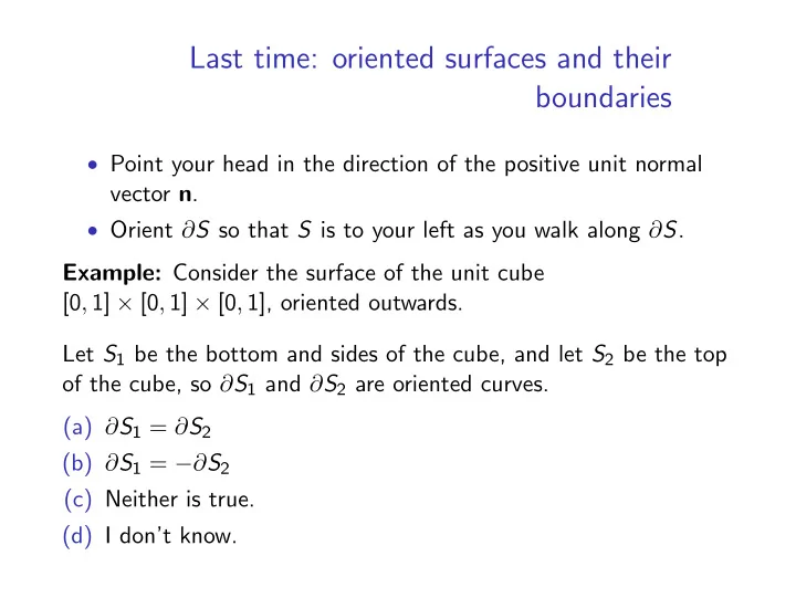
∙ Point your head in the direction of the positive unit normal
vector n.
∙ Orient ∂S so that S is to your left as you walk along ∂S.
Example: Consider the surface of the unit cube [0, 1] × [0, 1] × [0, 1], oriented outwards. Let S1 be the bottom and sides of the cube, and let S2 be the top
- f the cube, so ∂S1 and ∂S2 are oriented curves.
(a) ∂S1 = ∂S2 (b) ∂S1 = −∂S2 (c) Neither is true. (d) I don’t know.
SLIDE 2
Announcements
∙ Deadline to request a regrade for midterm 3 is this Thursday. ∙ Final exam is next Friday. (!) I will organize some kind of
review session next Wednesday/Thursday/Friday. Fill out the survey on the course webpage indicating your availability if you’re interested.
SLIDE 3 More on Stokes’ Theorem and Curl
Recall:
∙ We assume we have a vector field F defined on some open
region D ⊂ R3, with continuous first order partial derivatives
∙ S is an oriented surface contained in D. We assume S is
“nice”:
- S is piecewise smooth.
- ∂S consists of one or more simple closed paths.
Theorem (Stokes’ Theorem)
∫︂∫︂
S
curl F · dS = ∫︂
∂S
F · dr.
SLIDE 4
More on Stokes’ Theorem and Curl
Let F be the velocity field of a fluid flow in R3. Choose a point P in R3, and choose any vector unit vector n at P. Let D be a small disk with centre P and unit normal n, and place a tiny paddle wheel at P with its axis of rotation in direction n. The counterclockwise force on the wheel is related to the circulation of F around ∂D: ∼ ∫︂
∂D
F · dr. But by Stokes’ theorem, this is ∫︂∫︂
D
curlF · n dA.
SLIDE 5
The counterclockwise force on the wheel is related to the circulation of F around ∂D: ∼ ∫︂
∂D
F · dr = ∫︂∫︂
D
curlF · n dA. We approximate the function curlF · n over the small disk D by its value at the centre point P.
∙ The wheel rotates counterclockwise if curlF · n > 0 at P. ∙ It rotates clockwise if curlF · n < 0 at P. ∙ It doesn’t rotate at all if curlF · n = 0.
The speed of rotation is related to |curl · n|. If we want to place a tiny wheel at P oriented so that it will spin as quickly as possible, we should choose the angle/direction n so that |curl · n| is as large as possible. i.e. we should choose n to be pointing in the same direction (±) as curl.
SLIDE 6
Analogy
If f is a function, the gradient ∇f (P) points in the direction we should face if we want to increase as quickly as possible. If F is a vector field, the curl ∇ × F(P) points in the direction we should stand if we want to be spun around as quickly as possible.
SLIDE 7
Practice with Stokes’ theorem: computing a hard surface integral by changing it into an easy surface integral
Let S be the blob drawn on the board, oriented outward, with boundary edges of the square [0, 1] × [0, 1] × {1}. Let F be as before. What is ∫︁∫︁
S curlF · dS?
(a) -1 (b) 0 (c) 1 (d) Not enough information. (e) I don’t know.
SLIDE 8
Practice with Stokes’ theorem
F = ⟨ y x2 + y2 , −x x2 + y2 , ez2⟩. This is defined everywhere except the z-axis, {x = y = 0}. Claim: curl F = ⃒ ⃒ ⃒ ⃒ ⃒ ⃒ i j k ∂x ∂y ∂z
y x2+y2 −x x2+y2
ez2 ⃒ ⃒ ⃒ ⃒ ⃒ ⃒ = 0.
SLIDE 9
ST: Converting a hard line integral to an easy surface integral
Let C1 be the curve parametrized by r1(θ) = ⟨4 cos θ − cos 4θ, 1, 4 sin θ − sin 4θ⟩, 0 ≤ θ ≤ 2π. Let S be the surface we get by filling in the curve in the y = 1 plane. Observe that S doesn’t intersect the z-axis, so F is defined on all of S. Orient S so that ∂S = C1. Then Stokes’ Theorem says: ∫︂
C1
F · dr = ∫︂∫︂
S
curlF · dS = 0.
SLIDE 10 More practice with Stokes’ Theorem
Let F be as before, but now let C2 be the curve parametrized by r2(θ) = ⟨4 cos θ − cos 4θ, 4 sin θ − sin 4θ, 1⟩, 0 ≤ θ ≤ 2π. Does the previous argument work to show that ∫︁
C2 F · dr = 0? Why
(a) No. (b) Yes.