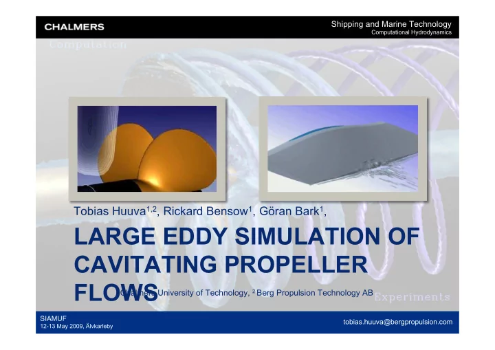
large eddy simulation of cavitating propeller flows
play

LARGE EDDY SIMULATION OF CAVITATING PROPELLER FLOWS 1 Chalmers - PowerPoint PPT Presentation

Shipping and Marine Technology Computational Hydrodynamics Tobias Huuva 1,2 , Rickard Bensow 1 , Gran Bark 1 , LARGE EDDY SIMULATION OF CAVITATING PROPELLER FLOWS 1 Chalmers University of Technology, 2 Berg Propulsion Technology AB SIAMUF


  1. Shipping and Marine Technology Computational Hydrodynamics Tobias Huuva 1,2 , Rickard Bensow 1 , Göran Bark 1 , LARGE EDDY SIMULATION OF CAVITATING PROPELLER FLOWS 1 Chalmers University of Technology, 2 Berg Propulsion Technology AB SIAMUF tobias.huuva@bergpropulsion.com 12-13 May 2009, Älvkarleby

  2. Shipping and Marine Technology Computational Hydrodynamics Background Requirements for numerical cavitation erosion predictions? • Which cavitation mechanism are necessary to include? – Side and re-entrant jets Supported by experimental observations – Importance of viscosity (EROCAV, Virtue) – Cloud formation – … • Computational requirements? – RANS vs. LES Supported by workshops, project – Mesh resolution meetings, private communication – Compressibility – … SIAMUF tobias.huuva@bergpropulsion.com 12-13 May 2009, Älvkarleby

  3. Shipping and Marine Technology Computational Hydrodynamics Modeling approach Incompressible, viscous LES with VoF – Probably beneficial to take compressibility into account • Solver stability, physical modeling, pressure pulse prediction – LES natural choice for cavitating flows • Inherently unsteady • Difference in computational cost compared with RANS not that large – Physics require fine resolution in time and space • Prospect of high frequency phenomena – Single fluid two-phase mixture works well with filtering in LES – Unstructured grids (Propeller) Instantaneous Time average • Local grid refinement necessary – Mass transfer model (“cavitation model”) • Less important than flow solver choices SIAMUF tobias.huuva@bergpropulsion.com 12-13 May 2009, Älvkarleby

  4. Shipping and Marine Technology Computational Hydrodynamics Computational Configuration – ILES in mixed formulation • 2 nd order backward differencing in time – Δ t ≈ 2e-6 • CD with limiter for convective terms • PISO – Mixed fluid – vapor/liquid • VoF-approach • Transport equation for vapor fraction α – Mass transfer modeling following Kunz • A + =1e6, A - =1e3, ρ l / ρ v =1000 with 1 – OpenFOAM • Open source CFD library tools 1 Huuva et al., IAHR symp. 2007 Huuva, PhD-thesis, 2008 SIAMUF tobias.huuva@bergpropulsion.com 12-13 May 2009, Älvkarleby

  5. Shipping and Marine Technology Computational Hydrodynamics LES Modeling – Mixed formulation 1 ( ) ( ) + ( ) B = v � v � v � v + v v + � v � v v � � v = L + C + R � � � ( ) ( ) ( ) % % % � � � � � � � � B v v v v v v v v v v v v v v v v L C R � � � � � � � � = � + � + � + � = + + – Implicit modeling • Physical dissipation represented by numerical dissipation • Flux limiting, dissipative numerical scheme – Wall modeling 2 • Law-of-the-wall based • Adjust viscosity to account for wall effects • Used both with explicit and implicit approaches • Extensively tested 1 Bensow & Fureby, J. Turbulence 8 :54, 2007 2 Fureby et al. AIAA J. 2004 SIAMUF tobias.huuva@bergpropulsion.com 12-13 May 2009, Älvkarleby

  6. Shipping and Marine Technology Computational Hydrodynamics Propeller flow validation • Non-cavitating, homogenous inflow – J=0.88: U ∞ =5 m/s, 25 rps 1 – 4.8M cells, tets+prisms – J=0.71: U ∞ =5.808 m/s, 36 rps – Refined in tip vortex and blade wake regions – D P =0.227 m J K T 10K Q η 0.88 Exp 0.157 0.306 0.719 Experiments by DiFelice et al., ||curl(U)||=75 ILES 0.158 0.308 0.718 MixedILES 0.157 0.308 0.714 MixedILES (limitedLinear) 0.159 0.307 0.725 MixedILES (no WM) 0.159 0.316 0.704 OEEVM 0.150 0.317 0.663 MixedOEEVM 0.153 0.320 0.668 0.71 Exp 0.256 0.464 0.623 MixedILES (limitedLinear) 0.256 0.453 0.639 1 Bensow & Liefvendahl AIAA 38 th Fluid Dyn., 2008 SIAMUF tobias.huuva@bergpropulsion.com 12-13 May 2009, Älvkarleby

  7. Shipping and Marine Technology Computational Hydrodynamics Propeller flow validation Normalized axial velocity @ x/R P =0.65 r/R P =0.25, 0.7, 0.95, 1.05 SIAMUF tobias.huuva@bergpropulsion.com 12-13 May 2009, Älvkarleby

  8. Shipping and Marine Technology Computational Hydrodynamics Delft Twist11 Foil • NACA009 with varying aoa, -2° to 9° • Similar to propeller blade root section Experiments by Foeth et al. • Unsteady cavitation in homogeneous inflow U ∞ =6.97 m/s, σ =1.07, L C =0.15m • • 2.2M cells, hex, half domain SIAMUF tobias.huuva@bergpropulsion.com 12-13 May 2009, Älvkarleby

  9. Shipping and Marine Technology Computational Hydrodynamics Delft Twist11 Foil, cont’… SIAMUF tobias.huuva@bergpropulsion.com 12-13 May 2009, Älvkarleby

  10. Shipping and Marine Technology Computational Hydrodynamics Cavitating E779A Propeller in Open Water • J=0.71, σ n =1.76 – U ∞ =5.808 m/s, 36 rps, D P =0.227 m SIAMUF tobias.huuva@bergpropulsion.com 12-13 May 2009, Älvkarleby

  11. Shipping and Marine Technology Computational Hydrodynamics E779A in Artificial Wake • J=0.90, σ n =4.455 – U ∞ =6.22 m/s, 30.5 rps, D P =0.227 m – Grid with 4.6 M cells, tets+prisms, locally refined in sheet cavity region SIAMUF tobias.huuva@bergpropulsion.com 12-13 May 2009, Älvkarleby

  12. Shipping and Marine Technology Computational Hydrodynamics Cavitation Dynamics Experiments by Pereira et al. SIAMUF tobias.huuva@bergpropulsion.com 12-13 May 2009, Älvkarleby

  13. Shipping and Marine Technology Computational Hydrodynamics Cavitation Dynamics Experiments by Pereira et al. SIAMUF tobias.huuva@bergpropulsion.com 12-13 May 2009, Älvkarleby

  14. Shipping and Marine Technology Computational Hydrodynamics Tip Vortex/Cavity interaction SIAMUF tobias.huuva@bergpropulsion.com 12-13 May 2009, Älvkarleby

  15. Shipping and Marine Technology Computational Hydrodynamics Conclusions • Possible to simulate some mechanisms of dynamic cavitation – Detect initial condition for erosive cavitation – Mesh resolution needs to be finer to trace shed cavities – Room for improvement in modeling but not essential – May soon be used for advanced design considerations • Numerical methods and physical modeling tightly coupled – These results are not credited to a single isolated factor (LES, Kunz, parameter settings etc.) SIAMUF tobias.huuva@bergpropulsion.com 12-13 May 2009, Älvkarleby

  16. Shipping and Marine Technology Computational Hydrodynamics Thanks for your attention! Questions and comments! Tobias Huuva tobias.huuva@bergpropulsion.com SIAMUF tobias.huuva@bergpropulsion.com 12-13 May 2009, Älvkarleby

Download Presentation
Download Policy: The content available on the website is offered to you 'AS IS' for your personal information and use only. It cannot be commercialized, licensed, or distributed on other websites without prior consent from the author. To download a presentation, simply click this link. If you encounter any difficulties during the download process, it's possible that the publisher has removed the file from their server.

Recommend


More recommend