Lagrangian Observations in the Atmosphere Balloons Horizontal - PowerPoint PPT Presentation

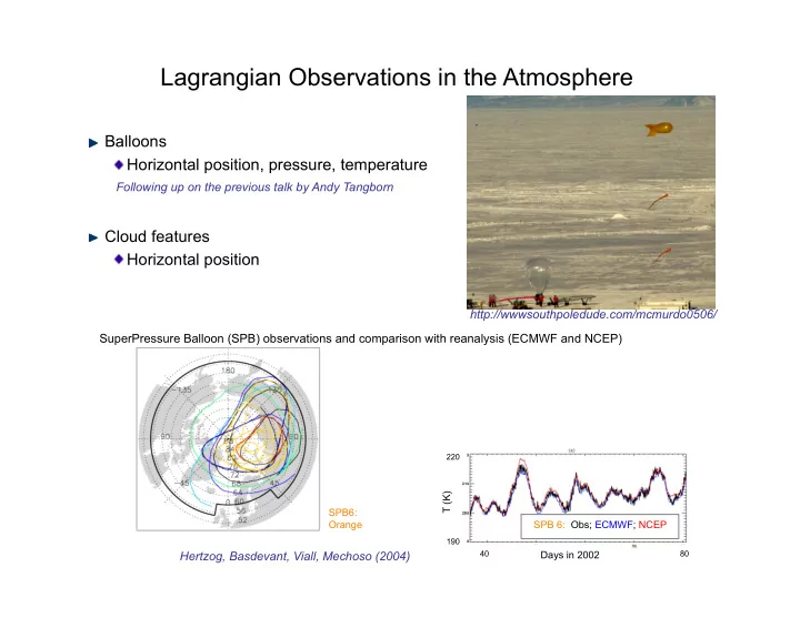
Lagrangian Observations in the Atmosphere Balloons Horizontal position, pressure, temperature Following up on the previous talk by Andy Tangborn Cloud features Horizontal position http://wwwsouthpoledude.com/mcmurdo0506/ SuperPressure Balloon (SPB) observations and comparison with reanalysis (ECMWF and NCEP) 220 T (K) SPB6: Orange SPB 6: Obs; ECMWF; NCEP 190 Hertzog, Basdevant, Viall, Mechoso (2004) 40 Days in 2002 80

Lagrangian Data Assimilation (LaDA): Method and Mathematical Challenges Kayo Ide, UCLA Guillaume Vernieres & Chris Jones, UNC-CH Hayder Salman, Cambridge Unversity Data available from http://www.aoml.noaa.gov/phod/dac/dacdata.html http://www.drifters.doe.gov/design.html

Two Mathematical Issues in LaDA 1. High nonlinear drifter dynamics  Handing of chaotic data 2. Limited number of observations  Deployment strategy

Basic Elements of Lagrangian Data Assimilation System ⎛ ⎞ ⎛ ⎞   ( ) ( ) ⎜ ⎟ ⎜ ⎟ ( x ) t k r D, j u ijl t k ⎜ ⎟ ⎜ ⎟ ( ) ( ) ( ) = ( ) = ( y ) t k ⎜ ⎟ ⎜ ⎟ r D, j x F t k v ijl t k y D, j t k ⎜ ⎟ ⎜ ⎟ ( ) ( ) ( p ) t k L D = 2 [or 3] N F  10 5-7 ⎜ ⎡ ⎤ ⎟ ⎜ ⎟ h ijl t k r D, j ⎣ ⎦ ⎜ ⎟ ⎜ ⎟ per drifter ⎝ ⎠  ⎝ ⎠  Application to Gulf of Mexico: Next Presentation by Guillaume Vernieres

Lagrangian Data Assimilation (LaDA) Method Eulerian Models x F Lagrangian Data y D Augmented model state x Partial observation y of x o = Hx t + ε D = x D t + ε D y D ⎛ ⎞ ⎛ ⎞ x F P ≡ P P x ≡ FF FD ⎜ ⎟ ⎜ ⎟ ⎝ x D ⎠ ⎝ P P ⎠ DF DD ( ) ( ) ( ) ( ) ε D  N 0 ( ) ⎛ ⎞ ⎛ ⎞ m F x F t k − 1 x F t k H = 0 I R DD o ⎟ = ⎜ ⎟ ⎜ ( ) ( ) ( ) , x D t k − 1 ( ) ⎜ ⎟ x D t k ⎝ ⎠ m D x F t k − 1 ⎝ ⎠ Lagrangian Data Assimilation Explicit computation of (LaDA) flow-dependent P is required Direct assimilation of y D into x F ⎛ ⎞ ⎛ ⎞ ⎛ ⎞ x F a x F f ⎟ + P f − 1 y D ( ) ( ) a = f + R DD o − x D ⎟ = x ⎟ P o f FD ⎜ ⎜ ⎜ ⎝ x D a ⎠ ⎝ x D f ⎠ ⎝ P f ⎠ DD DD EKF: Ide, Jones, Kuznetsov (2002); EnKF: Salman,Kuznetsov, Jones, Ide (2005)

Proof of Concept: Application to Mid-latitude Ocean Circulation Ocean circulation Perfect model scenario 1-layer shallow-water model Model spin-up for 12yrs Wind-driven: τ =0.05 Ns -2 Nature run with H 0 =500m Domain size: 2000km x 2000km Ensemble with (H mean , H std )=(550m,50m) Drifters Released at the beginning of 13yr Observed every day with σ std =200m

Case: ν = 500m 2 s -1 , ( ∆ T , L D )=(1day, 1) Background color contour: instantaneous h Truth With LaDA Without DA Analysis Ensemble Mean T=0 days Trajectory for 90days T=90 days Weakly chaotic ocean dynamics by basin-scale Rossby wave

Case: ν = 500m 2 s -1 , ( ∆ T , L D )=(1day, 1) Truth With LaDA Without DA Analysis Ensemble Mean T=0 days T=90 days

Issue 1: Handling of Chaotic Data for x D Spatially-Temporally chaotic ocean dynamics in truth: ν =400 m 2 s -1 Triangles in color: Drifters motion in truth Curves in purple: Material boundaries (manifolds for x D ) Background contour: Instantaneous h in truth

Sudden Filter Divergence by the Hyperbolic Effect for x D Ensemble spread of x D ( Δ T=20) Ensemble mean (forecast/analysis) x D ( t =0) x D ( t =40) f x D o − x d = y f D Hyperbolic Trajectory (HT) x D ( t =20) a x o y D D Large innovation d can occur near a hyperbolic trajectory(HT) Spread of P f DD brings x a D properly close to y o Unreastically large Δ x f D can occur due to poor representation of P f FD ⎛ Δ x F ⎞ ⎛ ⎞ ⎟ = P a f ( f + R D ) − 1 d ⎟ P FD o ⎜ ⎜ ⎝ Δ x D ⎠ ⎝ ⎠ DD P a f DD

Quality Control Scheme to Handle Chaotic Data for x D Two potential sources for large d = y o – x D t 1. Large observation error: y o – x D t  No update (outlier y o ) 2. Fast dispersion in: x D f – x D t  Update at least x D & check for x F Outline of the quality control scheme a) Detection of hyperbolic effect (HE) in x D f using 2 tests Update with QC Scheme 1. Against R d o : o = d ( ) T R D − 1 d of ≥ β o of < β o C D C D c D o o < β o C D x F & x D x F & x D 2. Against ( P DD f + R D o ): o ≥ β o C D No Update HE detected of = d ( f + R D ) T P − 1 d c D o DD a < β a a ≥ β a C F C F Sanity check for Δ x F b) a x F & x D x D only 1. Against P FF f : a T P a = Δ x F ( ) − 1 Δ x F c F f a FF More sophisticated approach (Particle filter): Spiller, Budhiraja, Ide, Jones (2008)

Issue 2: Towards Observing System Design Observing system: Trajectories significantly differ depending on deployment locations/times Once Lagrangian instruments are released, they go with the flow. Number of drifters and resources to deploy instruments are limited. Data assimilation system: Regions where Lagrangian observations effectively correct the model state are restricted around the trajectories. Observing system design = targeting (without metric) by taking into account of Lagrangian flow structures evolving in { x F ( t )} Freely moving instruments { x D ( t )} in { x F ( t )}

Directed Deployment of Drifters for Targeting in x F for x D Eddy tracking Deploy so that drifters will stay in the eddy Survey of largest possible area Deploy where drifters will spread out quickly visit various parts of the flow Balanced performance Use combination If no information about Lagrangian flow dynamics Deploy uniformly or based on educated guesses (and cross your fingers)

Lagrangian Flow Template by Dynamical Systems Theory Stable and unstable manifolds from the hyperbolic trajectories (HTs) = “material boundaries” of distinct Lagrangian flow regions Dynamical systems theory: A tool analyze Lagrangian dynamics given a time sequence of (Eulerian) flow field Eulerian Model Field Lagrangian flow template for { x F ( t ), t 0 -T ≤ t ≤ t 0 -T } { x D ( t 0 )} Dynamical Systems Theory How to detect manifolds? How to obtain Lagrangian flow template?

Lagrangian Flow Template for x D in Unsteady Flow x F Direct Lyapunov Exponents (DLE): divergence of the nearby trajectories ( ) ≈ x D t 0 + T ; x 0 ,t 0 ( ) + δ x D t 0 + T ; x 0 ,t 0 ( ) x D t 0 + T ; x 0 + δ x 0 ,t 0 { } δ x 0 ( ) ( ) = exp σ t; x 0 ,t 0 ( ) max δ x 0 δ x D t 0 + T ; x 0 ,t 0 σ t; x 0 ,t 0 DLE : forward DLE ( T >0) → stable manifolds High divergence: backward DLE ( T <0) → unstable manifolds High values of DLE (gray: T <0) and (red: T <0) at t 0 =0 with T =10days stable manifold Unstable manifold Background contour: instantaneous h Application to transport: Haller (2001, 2002) and Others. Application to DA: Salman, Ide, Jones (2007) Reconstruction of velocity field: Poje, Toner, Kirwan, Jones (2002)

Targeting based on Lagrangian Flow Template (Manifolds) Local targeting : Eddy tracking ⇒ Deploy inside of eddy, surrounded by the stable & unstable manifolds Global targeting: Survey of the largest possible area ⇒ Deploy both side of the stable manifolds for fastest divergence along the unstable manifolds ⇒ Deploy into the jet/current defined by the manifolds Mixed strategy : Balanced performance ⇒ Deploy using local & global targeting Mixed strategy Lagrangian flow template Targeting

Observing System Design for Mid-Latitude Ocean Perfect model scenario Model spin-up for 12yrs Nature run with h 0 =500m Ensemble with ( h mean , h std )=(550m,50m) Drifters Released at the beginning of 13yr Observed every day with σ std =200m Test strategies using 9 drifters Uniform Global Targeting Local Targeting Mixed Strategy Deployment (3 HT x 3) (3 eddies x 3) (3 eddies x 1 (3 x 3) 2 HT x 3)

Local Targeting Strategy T=25days T=100days T=300days Truth Local Initial error in h: Global targeting Failure to capture new eddy generation Background color contour: instantaneous h

Global Targeting Strategy T=25days T=100days T=300days Truth Global targeting

Mixed Strategy = Global + Local T=25days T=100days T=300days Truth Mixed

Spatial Distribution of RMSE in h T=25days T=100days T=300days Local Targeting Failure to capture new eddy generation Global Targeting Effective basin-scale estimation by fast divergence

Spatial Distribution of RMSE in h T=25days T=100days T=300days Mixed Strategy Uniform Deployment

Spatial Distribution of RMSE in KE T=25days T=100days T=300days Local Initial KE error distribution: local Targeting Failure to capture new eddy generation Global Targeting

Spatial Distribution of RMSE in KE T=25days T=100days T=300days Mixed strategy Uniform Deployment

Remarks on Deployment Strategy Deployment strategy It is targeting for x D ( t 0 ), using Lagrangian flow template obtained by { x F ( t ), t 0 -T ≤ t ≤ t 0 +T } It is naturally built on dynamical systems theory Eulerian Model Field Lagrangian flow template Directed Deployment { x F ( t ), t 0 -T ≤ t ≤ t 0 -T } x D ( t 0 ) (e.g., Mixed strategy) DLE / dynamical systems theory Targeting