Lagged Regression again: Transfer Functions To forecast an output - PowerPoint PPT Presentation

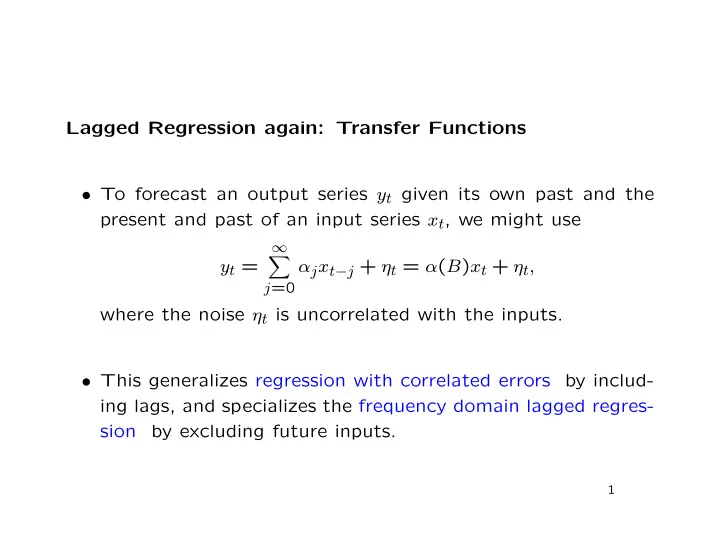
Lagged Regression again: Transfer Functions • To forecast an output series y t given its own past and the present and past of an input series x t , we might use ∞ � y t = α j x t − j + η t = α ( B ) x t + η t , j =0 where the noise η t is uncorrelated with the inputs. • This generalizes regression with correlated errors by includ- ing lags, and specializes the frequency domain lagged regres- sion by excluding future inputs. 1

• Preliminary estimation of α 0 , α 1 , . . . often suggests a parsi- monious model α ( B ) = B d × δ ( B ) ω ( B ) , where: – d is the pure delay : α 0 ≈ α 1 ≈ · · · ≈ α d − 1 ≈ 0 and α d � = 0; – δ ( B ) and ω ( B ) are low-order polynomials: ω ( B ) is needed if the α ’s decay exponentially, and δ ( B ) is needed if the first few nonzero α ’s do not follow the decay. • Preliminary estimates from frequency domain method, or a similar time domain method. 2

Time Domain Preliminary Estimates • If the input series x t were white noise, the cross correlation � � γ y,x ( h ) = E y t + h x t     ∞ �  x t    = E α j x t + h − j + η t + h j =0 = α h var ( x t ) , γ y,x ( h ) / � so ˆ var ( x t ) provides an estimate of α h . • Usually, x t is not white noise, but if it is a stationary time series, we know how to make it white: fit an ARMA model. 3

Prewhitening • Suppose that x t is ARMA: φ ( B ) x t = θ ( B ) w t , where w t is white noise. • Apply the prewhitening filter φ ( B ) θ ( B ) − 1 to the lagged re- gression equation: ∞ � y t = ˜ α j w t − j + ˜ η t , j =0 y t = [ φ ( B ) θ ( B ) − 1 ] y t and ˜ η t = [ φ ( B ) θ ( B ) − 1 ] η t . where ˜ 4

• Now the cross correlation γ ˜ y,w ( h ) provides an estimate of α h . • You can use SAS’s proc arima to do this: – first identify and estimate a model for x t ; – then identify y t with x t as a crosscorr variable. At the second step, SAS uses the prewhitening filter from the first step to filter both x t and y t before calculating cross correlations. • Note: SAS announces that both series have been “prewhitened”, but the filter is designed to prewhiten only x t ; y t is filtered , but typically not prewhitened. 5

• Finally estimate the model for y t , specifying the input series, in the form: input = ( d $( L 1 , 1 , L 1 , 2 , . . . ) . . . ( L k, 1 , . . . ) / ( L k +1 , 1 , . . . ) . . . ( . . . )variable) • E.g. for Southern Oscillation and the fisheries recruitment series: program and output. • E.g. for global temperature and an estimated historical forc- ing series: program and output. 6

Interpreting a Transfer Function • For the global temperature case, we have y t = 0 . 087917 × ( x t +0 . 79513 x t − 1 +0 . 79513 2 x t − 2 + . . . )+ η t . • So the effect of an impulse in the forcing x t , say a dip due to a volcanic eruption, is felt in the current year and several subsequent years, with a mean delay of 1 / (1 − 0 . 79513) ≈ 4 . 9 years. 7

• Also, the effect of a sustained change of +4 . 4 W/m 2 would be 0 . 087917 × 4 . 4 × (1 + 0 . 79513 + 0 . 79513 2 + . . . ) = 0 . 087917 × 4 . 4 / (1 − 0 . 79513) ≈ 1 . 9 ◦ C . • This is the expected forcing for a doubling of CO 2 over pre- industrial levels, and the temperature response is called the climate sensitivity . The IPCC states: Analysis of models together with constraints from observations suggest that the equilibrium climate sen- sitivity is likely to be in the range 2 ◦ C to 4 . 5 ◦ C, with a best estimate value of about 3 ◦ C. It is very unlikely to be less than 1 . 5 ◦ C. 8

• Our estimate is at the low end of that range, but quantifying its uncertainty is difficult using proc arima . • The profile likelihood for climate sensitivity, constructed us- ing a grid search in R (with p = 4), gives an estimated value of 1 . 85 ◦ C and 95% confidence limits of 1 . 44 ◦ C to 2 . 27 ◦ C. 9

-2 Log-Likelihood contours for climate sensitivity (y-axis) and decay factor (x-axis): 2.5 2.0 1.5 0.4 0.5 0.6 0.7 0.8 0.9 10

-2 Log-Likelihood profile for climate sensitivity: −302 −304 −306 ll2 −308 −310 1.5 2.0 2.5 4.4 * theta 11

-2 Log-Likelihood profile for decay factor: −300 −302 −304 ll2 −306 −308 −310 0.4 0.5 0.6 0.7 0.8 0.9 lambda 12