L 1p p B A Constraints: Rational preferences Idea: preferences - - PDF document

SLIDE 1 ✁ ✂ ✄ ☎✆ ✝✞ ✂ ✟ ☎ ✁ ✂ ☎ ✠ ✄ ✂ ✟✡ ✞ ✟ ☛ ☞ ✁ ✂✌ ☞ ☞ ✟ ✍ ✌ ✁ ✞ ✌ ✎ ✏ ✑ ✒ ✓ ✔ ✏ ✕ ✖✗ ✘ ✒ ✙ ✒ ✓ ✔ ✙ ✚ ✛ ✜ ✢ ✣✤ ✥✦ ✧ ★ ✩✪✫ ✪✬ ✭ ✮✯ ✰ ✱✲✳✴ ✵ ✶✷ ✸✹ ✷ ✺ ✻✼ ✴ ✳ ✲ ✽ ✾ ✺ ✿ ❀ ❁ ✲ ✲ ✳ ✻ ✻ ✱ ✶ ✴ ❂ ✿❃ ✵ ❄ ❅ ✼ ❆ ❇ ❈ ❉ ❉❊ ❋

• ✱

❍ ■ ✳ ❄ ❈ ❏ ❑ ▲ ❑ ▼ ✝ ✂ ☞ ✟ ✁ ✌ ◆

Rational preferences

◆

Utilities

◆

Money

◆

Multiattribute utilities

◆

Decision networks

◆

Value of information

✰ ✱✲✳✴ ✵ ✶✷ ✸✹ ✷ ✺ ✻✼ ✴ ✳ ✲ ✽ ✾ ✺ ✿ ❀ ❁ ✲ ✲ ✳ ✻ ✻ ✱ ✶ ✴ ❂ ✿❃ ✵ ❄ ❅ ✼ ❆ ❇ ❈ ❉ ❉❊ ❋

• ✱

❍ ■ ✳ ❄ ❈ ❏ ❈ ▲ ❈ ❖ ✄ ✌ P ✌ ✄ ✌ ✁ ✞ ✌◗

An agent chooses among prizes (

❘

,

❙

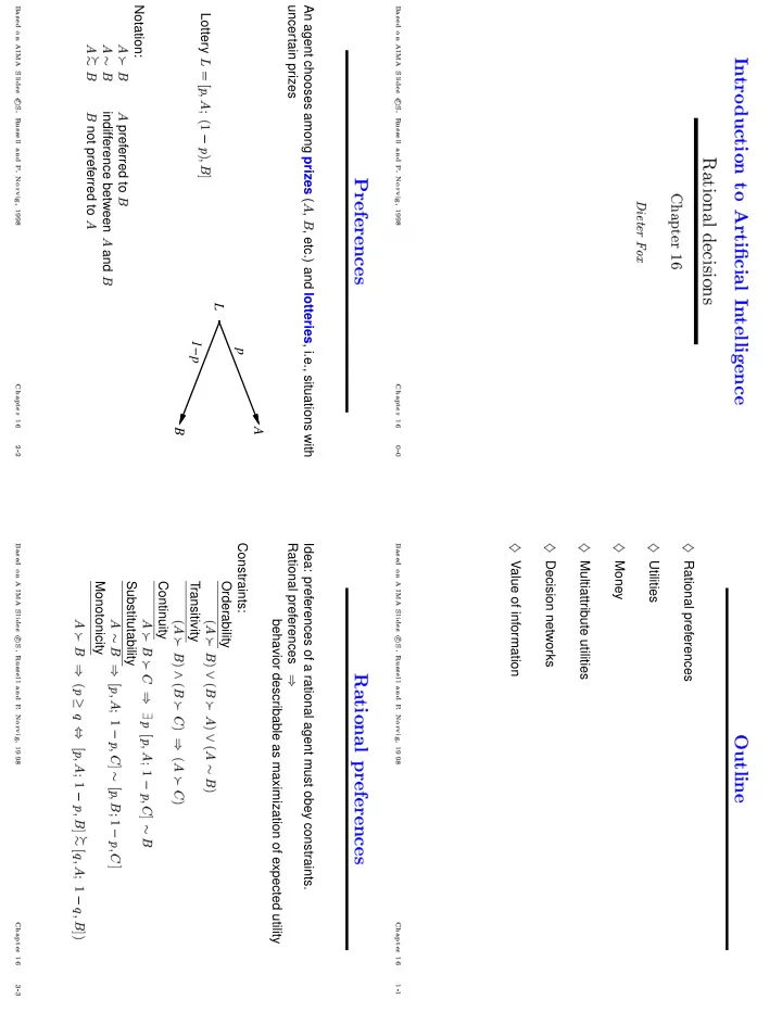
, etc.) and lotteries, i.e., situations with uncertain prizes Lottery

❚ ❯ ❱ ❲❳ ❘ ❨ ❩❭❬ ❪ ❲ ❫ ❳ ❙ ❴

L p 1−p A

❵

B

Notation:

❘ ❛ ❙ ❘

preferred to

❙ ❘ ❜ ❙

indifference between

❘

and

❙ ❘ ❛ ❜ ❙ ❙

not preferred to

❘ ✰ ✱✲✳✴ ✵ ✶✷ ✸✹ ✷ ✺ ✻✼ ✴ ✳ ✲ ✽ ✾ ✺ ✿ ❀ ❁ ✲ ✲ ✳ ✻ ✻ ✱ ✶ ✴ ❂ ✿❃ ✵ ❄ ❅ ✼ ❆ ❇ ❈ ❉ ❉❊ ❋

• ✱

❍ ■ ✳ ❄ ❈ ❏ ❝ ▲ ❝ ❞ ☛ ✂ ✟ ☎ ✁ ☛ ☞ ❡ ✄ ✌ P ✌ ✄ ✌ ✁ ✞ ✌◗

Idea: preferences of a rational agent must obey constraints. Rational preferences

❢

behavior describable as maximization of expected utility Constraints: Orderability

❩ ❘ ❛ ❙ ❫ ❣ ❩ ❙ ❛ ❘ ❫ ❣ ❩ ❘ ❜ ❙ ❫

Transitivity

❩ ❘ ❛ ❙ ❫ ❤ ❩ ❙ ❛ ✐ ❫ ❢ ❩ ❘ ❛ ✐ ❫

Continuity

❘ ❛ ❙ ❛ ✐ ❢ ❥ ❲ ❱ ❲❳ ❘ ❨ ❬ ❪ ❲❳ ✐ ❴ ❜ ❙

Substitutability

❘ ❜ ❙ ❢ ❱ ❲❳ ❘ ❨ ❬ ❪ ❲ ❳ ✐ ❴ ❜ ❱ ❲❳ ❙ ❨ ❬ ❪ ❲❳ ✐ ❴

Monotonicity

❘ ❛ ❙ ❢ ❩ ❲ ❦ ❧ ♠ ❱ ❲❳ ❘ ❨ ❬ ❪ ❲ ❳ ❙ ❴ ❛ ❜ ❱ ❧ ❳ ❘ ❨ ❬ ❪ ❧ ❳ ❙ ❴ ❫ ✰ ✱✲✳✴ ✵ ✶✷ ✸✹ ✷ ✺ ✻✼ ✴ ✳ ✲ ✽ ✾ ✺ ✿ ❀ ❁ ✲ ✲ ✳ ✻ ✻ ✱ ✶ ✴ ❂ ✿❃ ✵ ❄ ❅ ✼ ❆ ❇ ❈ ❉ ❉❊ ❋

• ✱

❍ ■ ✳ ❄ ❈ ❏ ♥ ▲ ♥

SLIDE 2 ❞ ☛ ✂ ✟ ☎ ✁ ☛ ☞ ❡ ✄ ✌ P ✌ ✄ ✌ ✁ ✞ ✌◗ ✞ ☎ ✁ ✂ ✆ ♦

Violating the constraints leads to self-evident irrationality For example: an agent with intransitive preferences can be induced to give away all its money If

❙ ❛ ✐

, then an agent who has

✐

would pay (say) 1 cent to get

❙

If

❘ ❛ ❙

, then an agent who has

❙

would pay (say) 1 cent to get

❘

If

✐ ❛ ❘

, then an agent who has

❘

would pay (say) 1 cent to get

✐

A

♣

B C

1c 1c 1c

✰ ✱✲✳✴ ✵ ✶✷ ✸✹ ✷ ✺ ✻✼ ✴ ✳ ✲ ✽ ✾ ✺ ✿ ❀ ❁ ✲ ✲ ✳ ✻ ✻ ✱ ✶ ✴ ❂ ✿❃ ✵ ❄ ❅ ✼ ❆ ❇ ❈ ❉ ❉❊ ❋

• ✱

❍ ■ ✳ ❄ ❈ ❏ q ▲ q r ☛ s ✟t ✟✉ ✟ ✁ ✍ ✌ s ❡ ✌ ✞ ✂✌ ✆ ✝ ✂ ✟ ☞ ✟ ✂ ✈

Theorem (Ramsey, 1931; von Neumann and Morgenstern, 1944): Given preferences satisfying the constraints there exists a real-valued function

✇

such that

✇ ❩ ❘ ❫ ❦ ✇ ❩ ❙ ❫ ♠ ❘ ❛ ❜ ❙ ✇ ❩ ❱ ❲ ① ❳ ② ① ❨ ③ ③ ③ ❨ ❲ ④ ❳ ② ④ ❴ ❫ ❯ ⑤ ⑥ ❲ ⑥ ✇ ❩ ② ⑥ ❫

MEU principle: Choose the action that maximizes expected utility Note: an agent can be entirely rational (consistent with MEU) without ever representing or manipulating utilities and probabilities E.g., a lookup table for perfect tictactoe

✰ ✱✲✳✴ ✵ ✶✷ ✸✹ ✷ ✺ ✻✼ ✴ ✳ ✲ ✽ ✾ ✺ ✿ ❀ ❁ ✲ ✲ ✳ ✻ ✻ ✱ ✶ ✴ ❂ ✿❃ ✵ ❄ ❅ ✼ ❆ ❇ ❈ ❉ ❉❊ ❋

• ✱

❍ ■ ✳ ❄ ❈ ❏⑦ ▲ ⑦ ⑧ ✂ ✟ ☞ ✟ ✂ ✟ ✌◗

Utilities map states to real numbers. Which numbers? Standard approach to assessment of human utilities: compare a given state

❘

to a standard lottery

❚ ⑨

that has “best possible prize”

⑩ ❶

with probability

❲

“worst possible catastrophe”

⑩ ❷

with probability

❩ ❬ ❪ ❲ ❫

adjust lottery probability

❲

until

❘ ❜ ❚ ⑨

L 0.999999 0.000001 continue as before instant death

pay $30 ~

✰ ✱✲✳✴ ✵ ✶✷ ✸✹ ✷ ✺ ✻✼ ✴ ✳ ✲ ✽ ✾ ✺ ✿ ❀ ❁ ✲ ✲ ✳ ✻ ✻ ✱ ✶ ✴ ❂ ✿❃ ✵ ❄ ❅ ✼ ❆ ❇ ❈ ❉ ❉❊ ❋

• ✱

❍ ■ ✳ ❄ ❈ ❏ ❏ ▲ ❏ ⑧ ✂ ✟ ☞ ✟ ✂ ✈ ◗ ✞ ☛ ☞ ✌◗

Normalized utilities:

⑩ ❶ ❯ ❬ ③ ❸

,

⑩ ❷ ❯ ❸ ③ ❸

Micromorts: one-millionth chance of death useful for Russian roulette, paying to reduce product risks, etc. QALYs: quality-adjusted life years useful for medical decisions involving substantial risk Note: behavior is invariant w.r.t. linear transformation

✇❺❹ ❩❼❻ ❫ ❯ ❽ ① ✇ ❩❼❻ ❫ ❾ ❽ ❿

where

❽ ① ➀ ❸

With deterministic prizes only (no lottery choices), only

• rdinal utility can be determined, i.e., total order on prizes

✰ ✱✲✳✴ ✵ ✶✷ ✸✹ ✷ ✺ ✻✼ ✴ ✳ ✲ ✽ ✾ ✺ ✿ ❀ ❁ ✲ ✲ ✳ ✻ ✻ ✱ ✶ ✴ ❂ ✿❃ ✵ ❄ ❅ ✼ ❆ ❇ ❈ ❉ ❉❊ ❋

• ✱

❍ ■ ✳ ❄ ❈ ❏➁ ▲ ➁

SLIDE 3 ➂ ✂ ✝ ✆ ✌ ✁ ✂ ✍ ✄ ☎ ✝ ❡ ✝ ✂ ✟ ☞ ✟ ✂ ✈

For each

❻

, adjust

❲

until half the class votes for lottery (M=10,000)

p $x 0.0 0.1 0.2 0.3 0.4 0.5 0.6 0.7 0.8 0.9 1.0 500 3000 4000 5000 6000 7000 8000 9000 10000 1000 2000

✰ ✱✲✳✴ ✵ ✶✷ ✸✹ ✷ ✺ ✻✼ ✴ ✳ ✲ ✽ ✾ ✺ ✿ ❀ ❁ ✲ ✲ ✳ ✻ ✻ ✱ ✶ ✴ ❂ ✿❃ ✵ ❄ ❅ ✼ ❆ ❇ ❈ ❉ ❉❊ ❋

• ✱

❍ ■ ✳ ❄ ❈ ❏ ❊ ▲ ❊ r ☎ ✁ ✌ ✈

Money does not behave as a utility function Given a lottery

❚

with expected monetary value

➃➄ ➅ ❩ ❚ ❫

, usually

✇ ❩ ❚ ❫ ➆ ✇ ❩ ➃➄ ➅ ❩ ❚ ❫ ❫

, i.e., people are risk-averse Utility curve: for what probability

❲

am I indifferent between a fixed prize

❻

and a lottery

❱ ❲❳ ➇ ➄ ❨ ❩ ❬ ❪ ❲ ❫ ❳ ➇ ❸ ❴

for large

➄

? Typical empirical data, extrapolated with risk-prone behavior:

+U +$

−150,000 800,000

• o o
• o o
• ✰

✱✲✳✴ ✵ ✶✷ ✸✹ ✷ ✺ ✻✼ ✴ ✳ ✲ ✽ ✾ ✺ ✿ ❀ ❁ ✲ ✲ ✳ ✻ ✻ ✱ ✶ ✴ ❂ ✿❃ ✵ ❄ ❅ ✼ ❆ ❇ ❈ ❉ ❉❊ ❋

• ✱

❍ ■ ✳ ❄ ❈ ❏ ❉ ▲ ❉ ➈ ✌ ✞ ✟ ◗ ✟ ☎ ✁ ✁ ✌ ✂➉ ☎ ✄➊ ◗

Add action nodes and utility nodes to belief networks to enable rational decision making

U Airport Site

Deaths Noise Cost Litigation Construction Air Traffic

Algorithm: For each value of action node compute expected value of utility node given action, evidence Return MEU action

✰ ✱✲✳✴ ✵ ✶✷ ✸✹ ✷ ✺ ✻✼ ✴ ✳ ✲ ✽ ✾ ✺ ✿ ❀ ❁ ✲ ✲ ✳ ✻ ✻ ✱ ✶ ✴ ❂ ✿❃ ✵ ❄ ❅ ✼ ❆ ❇ ❈ ❉ ❉❊ ❋

• ✱

❍ ■ ✳ ❄ ❈ ❏ ❈ ❑ ▲ ❈ ❑ r ✝ ☞ ✂ ✟ ☛ ✂ ✂ ✄ ✟ ➋ ✝ ✂✌ ✝ ✂ ✟ ☞ ✟ ✂ ✈

How can we handle utility functions of many variables

➌ ① ③ ③ ③ ➌ ④

? E.g., what is

✇ ❩❭➍ ➎➏➐➑ ➒ ❳ ➓ ➔→ ➒ ➎ ❳ ✐ ➔ ➒ ➐ ❫

? How can complex utility functions be assessed from preference behaviour? Idea 1: identify conditions under which decisions can be made without com- plete identification of

✇ ❩❼❻ ① ❳ ③ ③ ③ ❳ ❻ ④ ❫

Idea 2: identify various types of independence in preferences and derive consequent canonical forms for

✇ ❩❼❻ ① ❳ ③ ③ ③ ❳ ❻ ④ ❫ ✰ ✱✲✳✴ ✵ ✶✷ ✸✹ ✷ ✺ ✻✼ ✴ ✳ ✲ ✽ ✾ ✺ ✿ ❀ ❁ ✲ ✲ ✳ ✻ ✻ ✱ ✶ ✴ ❂ ✿❃ ✵ ❄ ❅ ✼ ❆ ❇ ❈ ❉ ❉❊ ❋

• ✱

❍ ■ ✳ ❄ ❈ ❏ ❈ ❈ ▲ ❈ ❈

SLIDE 4 ➂ ✂ ✄ ✟ ✞ ✂ ✆ ☎ t ✟ ✁ ☛ ✁ ✞ ✌

Typically define attributes such that

✇

is monotonic in each Strict dominance: choice

❙

strictly dominates choice

❘

iff

➣ → ➌ ⑥ ❩ ❙ ❫ ❦ ➌ ⑥ ❩ ❘ ❫

(and hence

✇ ❩ ❙ ❫ ❦ ✇ ❩ ❘ ❫

)

1

X

2

X A B C D

1

X

2

X A B C

This region dominates A Deterministic attributes Uncertain attributes

Strict dominance seldom holds in practice

✰ ✱✲✳✴ ✵ ✶✷ ✸✹ ✷ ✺ ✻✼ ✴ ✳ ✲ ✽ ✾ ✺ ✿ ❀ ❁ ✲ ✲ ✳ ✻ ✻ ✱ ✶ ✴ ❂ ✿❃ ✵ ❄ ❅ ✼ ❆ ❇ ❈ ❉ ❉❊ ❋

• ✱

❍ ■ ✳ ❄ ❈ ❏ ❈ ❝ ▲ ❈ ❝ ↔ ☛ ☞ ✝ ✌ ☎ P ✟ ✁ P ☎ ✄ t ☛ ✂ ✟ ☎ ✁

Idea: compute value of acquiring each possible piece of evidence Can be done directly from decision network Example: buying oil drilling rights Two blocks

❘

and

❙

, exactly one has oil, worth

❽

Prior probabilities 0.5 each, mutually exclusive Current price of each block is

❽ ↕❭➙

Consultant offers accurate survey of

❘

. Fair price? Solution: compute expected value of information = expected value of best action given the information minus expected value of best action without information Survey may say “oil in A” or “no oil in A”, prob. 0.5 each = [

❸ ③ ➛ ➜

value of “buy A” given “oil in A” +

❸ ③ ➛ ➜

value of “buy B” given “no oil in A”] – 0 =

❩ ❸ ③ ➛ ➜ ❽ ↕ ➙ ❫ ❾ ❩ ❸ ③ ➛ ➜ ❽ ↕❭➙ ❫ ❪ ❸ ❯ ❽ ↕❭➙ ✰ ✱✲✳✴ ✵ ✶✷ ✸✹ ✷ ✺ ✻✼ ✴ ✳ ✲ ✽ ✾ ✺ ✿ ❀ ❁ ✲ ✲ ✳ ✻ ✻ ✱ ✶ ✴ ❂ ✿❃ ✵ ❄ ❅ ✼ ❆ ❇ ❈ ❉ ❉❊ ❋

• ✱

❍ ■ ✳ ❄ ❈ ❏ ❈ ♥ ▲ ❈ ♥ ➝ ✌ ✁ ✌ ✄ ☛ ☞ P ☎ ✄ t ✝ ☞ ☛

Current evidence

➃

, current best action

➞

Possible action outcomes

② ⑥

, potential new evidence

➃ ➟ ➃ ✇ ❩ ➞ ➠ ➃ ❫ ❯ ➡ ➢ ➤ ➥ ⑤ ⑥ ✇ ❩ ② ⑥ ❫❭➦ ❩ ② ⑥ ➠ ➃ ❳ ➏ ❫

Suppose we knew

➃ ➟ ❯ ➎ ➟ ➧

, then we would choose

➞ ➨ ➩ ➫

s.t.

➃ ✇ ❩ ➞ ➨ ➩ ➫ ➠ ➃ ❳ ➃ ➟ ❯ ➎ ➟ ➧ ❫ ❯ ➡ ➢ ➤ ➥ ⑤ ⑥ ✇ ❩ ② ⑥ ❫ ➦ ❩ ② ⑥ ➠ ➃ ❳ ➏ ❳ ➃ ➟ ❯ ➎ ➟ ➧ ❫ ➃ ➟

is a random variable whose value is

➭➯ ✬ ✬ ✪➲ ✫➳ ➵

unknown

❢

must compute expected gain over all possible values:

➅ ➦➸ ➺ ❩ ➃ ➟ ❫ ❯ ➻ ⑤ ➧ ➦ ❩ ➃ ➟ ❯ ➎ ➟ ➧ ➠ ➃ ❫ ➃ ✇ ❩ ➞ ➨ ➩ ➫ ➠ ➃ ❳ ➃ ➟ ❯ ➎ ➟ ➧ ❫ ➼ ❪ ➃ ✇ ❩ ➞ ➠ ➃ ❫

(VPI = value of perfect information)

✰ ✱✲✳✴ ✵ ✶✷ ✸✹ ✷ ✺ ✻✼ ✴ ✳ ✲ ✽ ✾ ✺ ✿ ❀ ❁ ✲ ✲ ✳ ✻ ✻ ✱ ✶ ✴ ❂ ✿❃ ✵ ❄ ❅ ✼ ❆ ❇ ❈ ❉ ❉❊ ❋

• ✱

❍ ■ ✳ ❄ ❈ ❏ ❈ q ▲ ❈ q ❖ ✄ ☎ ❡ ✌ ✄ ✂ ✟ ✌◗ ☎ P ↔ ❖

• Nonnegative—in expectation, not post hoc

➣ ➽ ❳ ➃ ➅ ➦➸ ➺ ❩ ➃ ➟ ❫ ❦ ❸

Nonadditive—consider, e.g., obtaining

➃ ➟

twice

➅ ➦➸ ➺ ❩ ➃ ➟ ❳ ➃ ➧ ❫ ➾ ❯ ➅ ➦➸ ➺ ❩ ➃ ➟ ❫ ❾ ➅ ➦➸ ➺ ❩ ➃ ➧ ❫

Order-independent

➅ ➦➸ ➺ ❩ ➃ ➟ ❳ ➃ ➧ ❫ ❯ ➅ ➦➸ ➺ ❩ ➃ ➟ ❫ ❾ ➅ ➦➸ ➺ ➚ ➺ ➩ ❩ ➃ ➧ ❫ ❯ ➅ ➦➸ ➺ ❩ ➃ ➧ ❫ ❾ ➅ ➦➸ ➺ ➚ ➺ ➫ ❩ ➃ ➟ ❫

Note: when more than one piece of evidence can be gathered, maximizing VPI for each to select one is not always optimal

❢

evidence-gathering becomes a sequential decision problem

✰ ✱✲✳✴ ✵ ✶✷ ✸✹ ✷ ✺ ✻✼ ✴ ✳ ✲ ✽ ✾ ✺ ✿ ❀ ❁ ✲ ✲ ✳ ✻ ✻ ✱ ✶ ✴ ❂ ✿❃ ✵ ❄ ❅ ✼ ❆ ❇ ❈ ❉ ❉❊ ❋

• ✱

❍ ■ ✳ ❄ ❈ ❏ ❈ ⑦ ▲ ❈ ⑦

SLIDE 5 ➪ ✝ ☛ ☞ ✟ ✂ ☛ ✂ ✟ ➶ ✌ ➋ ✌ ➹ ☛ ➶ ✟ ☎ ✄ ◗

a) Choice is obvious, information worth little b) Choice is nonobvious, information worth a lot c) Choice is nonobvious, information worth little

P ( U | E )

j

➘

P ( U | E )

j

➘

P ( U | E )

j

➘

(a) (b) (c)

U U U U

1

U

2

U

2

U

2

U

1

U

1

✰ ✱✲✳✴ ✵ ✶✷ ✸✹ ✷ ✺ ✻✼ ✴ ✳ ✲ ✽ ✾ ✺ ✿ ❀ ❁ ✲ ✲ ✳ ✻ ✻ ✱ ✶ ✴ ❂ ✿❃ ✵ ❄ ❅ ✼ ❆ ❇ ❈ ❉ ❉❊ ❋

• ✱

❍ ■ ✳ ❄ ❈ ❏ ❈ ❏ ▲ ❈ ❏