Kinematic Redundancy A manipulator may have more DOFs than are - PowerPoint PPT Presentation

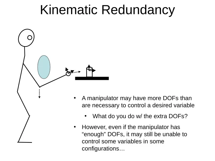
Kinematic Redundancy • A manipulator may have more DOFs than are necessary to control a desired variable • What do you do w/ the extra DOFs? • However, even if the manipulator has “enough” DOFs, it may still be unable to control some variables in some configurations…

Jacobian Range Space Before we think about redundancy, let’s look at the range space of the Jacobian transform: The velocity Jacobian maps joint velocities onto end ( ) q effector velocities:  = v J q v ( ) → J v q : Q V Space of joint velocities Space of end effector velocities • This is the domain of ( ) D J • J : This is the range v ( ) R J space of J : v

Jacobian Range Space ( ) → J v q : Q V In some configurations, the range space of the Jacobian may not span the entire space of the variable to be controlled: ( ( ) ) ∃ ∈ ∉ R v V , v J q v ( ( ) ) ( ( ) ) R ∀ ∈ ∈ R J v q v V , v J q spans if V v a Example: a and b span this two dimensional space: b

Jacobian Range Space This is the case in the manipulator to the right: • In this configuration, the Jacobian does not span the y direction (or the z direction) ( ( ) ) ∈ , ∉ R y V y J q v y x z

Jacobian Range Space Let’s calculate the velocity Jacobian: − l s − l s − l s − l s − l s − l s   1 1 2 12 3 123 2 12 3 123 3 123   ( ) = + + + J v q l c l c l c l c l c l c   1 1 2 12 3 123 2 12 3 123 3 123   0 0 0    π   2  q = 0   Joint configuration of manipulator: y   π   x − l − l + l − l + l l z   1 2 3 2 3 3   ( ) = J v q 0 0 0     0 0 0   ( ) q  q  = y J q There is no joint velocity, , that will produce a y velocity, v Therefore, you’re in a singularity.

Jacobian Singularities In singular configurations: J v ( q ) • does not span the space of Cartesian velocities J v ( q ) • loses rank y Test for kinematic singularity: [ ] x T det J ( q ) J ( q ) • If is zero, then manipulator is in z a singular configuration Example: − l − l + l 0   1 2 3 − − + − + l l l l l l something 0 [ ]       1 2 3 2 3 3 T = − + = det J ( q ) J ( q ) det l l 0 det       2 3 0 0 0 0 0       l 0   3 = 0

Jacobian Singularities: Example The four singularities of the three-link planar arm:

Jacobian Singularities and Cartesian Control Cartesian control involves calculating the inverse or pseudoinverse: ( ) T JJ − 1 # T = J J However, in singular configurations, the pseudoinverse (or inverse) does not exist ( ) − 1 T JJ because is undefined. y As you approach a singular configuration, joint x velocities in the singular direction calculated by z the pseudoinverse get very large: ( ) − 1  #  T T  = = = q J x J JJ x big s s In Jacobian transpose control, joint velocities in the singular direction ( i.e. the gradient) go to zero: T x    x = = q J 0 Where is a singular direction. s s

Jacobian Singularities and Cartesian Control • So, singularities are mostly a problem for Jacobian pseudoinverse control where the pseudoinverse “blows up”. • Not much of a problem for transpose control • The worst that can happen is that the manipulator gets “stuck” in a singular configuration because the direction of the goal y is in a singular direction. x • This “stuck” configuration is unstable – any z motion away from the singular configuration will allow the manipulator to continue on its way.

Jacobian Singularities and Cartesian Control One way to get the “best of both worlds” is to use the “dampled least squares inverse” – aka the singularity robust (SR) inverse: ( ) − 1 * T T 2 = + J J JJ k I • Because of the additional term inside the inversion, the SR inverse does not blow up. y • In regions near a singularity, the SR inverse trades x off exact trajectory following for minimal joint z velocities. BTW, another way to handle singularities is simply to avoid them – this method is preferred by many • More on this in a bit…

Kinematic redundancy 3 x A general-purpose robot arm frequently has 3 y more DOFs than are strictly necessary to l 3 l q 2 perform a given function 2 3 x 1 x 1 y q • in order to independently control the position 2 of a planar manipulator end effector, only 2 y 0 y two DOFs are strictly necessary q 1 0 x l • If the manipulator has three DOFs, then 1 0 z it is redundant w.r.t. the task of controlling two dimensional position. y x 2 2 y 3 • In order to independently control end q 3 l effector position in 3-space, you need at z y 3 2 1 least 3 DOFs z l 2 3 x q x 3 2 • In order to independently control end 1 z l effector position and orientation, at least 6 1 1 z 0 DOFs are needed (they have to be q 1 x configured right, too…) 0 y 0

Kinematic redundancy 3 x 3 y The local redundancy of an arm can be l 3 understood in terms of the local Jacobian l q 2 2 3 x 1 x 1 y • The manipulator controls a number of q 2 Cartesian DOFs equal to the number of 2 y independent rows in the Jacobian 0 y q 1 0 x l 1 j j j 0   z 11 12 13 = J   Since there are two independent j j j   rows, you can control two 21 22 23 Cartesian DOFs independently ( m =2) You use three joints to control two Cartesian DOFs ( n =3) Since the number of independent Cartesian directions is less than the number of joints, ( m<n ), this manipulator is redundant w.r.t. the task of controlling those Cartesian directions.

Kinematic redundancy 3 x 3 y What does this redundant space look like? l 3 l q • At first glance, you might think that it’s 2 2 3 x 1 x 1 y linear because the Jacobian is linear q 2 • But, the Jacobian is only locally linear 2 y 0 y q 1 0 x l The dimension of the redundant space is the 1 0 z number of joints – the number of independent Cartesian DOFs: n-m. • For the three link planar arm, the redundant space is a set of one dimensional curves traced through the three dimensional joint space. • Each curve corresponds to the set of joint configurations that place the end effector in Redundant manifolds in the same position. joint space

Kinematic redundancy 3 x Joint velocities in redundant directions 3 y causes no motion at the end effector l 3 l q 2 2 3 x 1 x • These are internal motions of the 1 y q manipulator. 2 2 y 0 y Redundant joint velocities satisfy this q 1 0 x l  equation: 0 = J ( q ) q 1 0 z J ( q ) the null space of { } ( )    = ∈ = N J ( q ) q Q : 0 J ( q ) q J ( q ) Compare to the range space of : { } ( )   Redundant manifolds in     = ∈ ∃ ∈ = R J ( q ) x X : q Q , x J ( q ) q joint space

Null space and Range space Joint space Cartesian space ( ) X ⊆ m R ⊆ − Q SO n 1   = x J ( q ) q ( ) R J ( q ) ( ) N J ( q ) You can’t generate { } ( )  these motions =  ∈ =  N J ( q ) q Q : 0 J ( q ) q { } Null space ( )   =  ∈ ∃  ∈  =  R J ( q ) x X : q Q , x J ( q ) q • Motions in the null space Range space are internal motions

Doing Things in the Redundant Joint Space 3 x 3 y Motions in the redundant space do not affect the l 3 l q 2 2 3 x 1 position of the end effector. x 1 y q 2 • Since they don’t change end effector 2 y 0 y position, is there something we would like to q 1 0 x do in this space? l 1 0 z • Optimize kinematic manipulability? • Stay away from obstacles? • Something else?

Doing Things in the Redundant Joint Space 3 x 3 y ( ) l 3  #  #  = + − q J x I J J q l q 2 2 3 x 1 x 0 1 y q 2 2 y 0 y q 1 0 x l 1 0 z − # I J J Null space projection matrix: • This matrix projects an arbitrary vector into the null space of J: Zero end-effector velocities • This makes it easy to do things in the redundant space – just calculate what you would like to do and project it into the null space.

Doing Things in the Redundant Joint Space 3 x 3 y l  q 3 Assume that you are given a joint velocity, , l q 0 2 2 3 x 1 x 1 you would like to achieve while also y q  2 x achieving a desired end effector twist, d 2 y 0 y  x • Required objective: q d 1 0 x l 1  q 0 z • Desired objective: 0 ( ) ( ) T      = − − f ( q ) q q q q 0 0  =  −  g ( q ) J q x = f ( z ) g ( z ) 0 Minimize subject to : ∇ = λ ∇ f ( z ) g ( z ) Use lagrange multiplier method: z z