
A Numerical Method
for Computing the
Jordan Canonical Form
Zhonggang Zeng, Northeastern Illinois Univ.
(Joint work with T. Y. Li, Michigan State Univ )
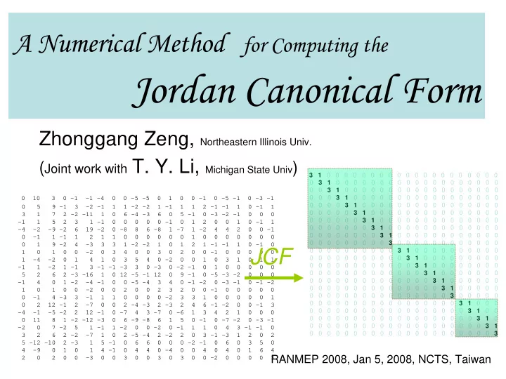
0 10 3 0 -1 -1 -4 0 0 -5 -5 0 1 0 0 -1 0 -5 -1 0 -3 -1 0 5 9 -1 3 -2 -1 1 1 -2 -2 1 -1 1 1 2 -1 -1 1 0 -1 1 3 1 7 2 -2 -11 1 0 6 -4 -3 6 0 5 -1 0 -3 -2 -1 0 0 0
- 1 1 5 2 3 1 -1 0 0 0 0 0 -1 0 1 2 0 0 1 0 -1 1
- 4 -2 -9 -2 6 19 -2 0 -8 8 6 -8 1 -7 1 -2 4 4 2 0 0 -1
0 -1 1 -1 1 2 1 1 0 0 0 0 0 0 1 0 0 0 0 0 0 0 0 1 9 -2 4 -3 3 3 1 -2 -2 1 0 1 2 1 -1 -1 1 0 -1 0 1 0 1 0 0 -2 0 3 4 0 0 3 0 2 0 0 -1 0 0 0 0 0 1 -4 -2 0 1 4 1 0 3 5 4 0 -2 0 0 1 0 3 1 0 1 1
- 1 1 -2 1 -1 3 -1 -1 -3 3 0 -3 0 -2 -1 0 1 0 0 0 0 0
5 2 6 2 -3 -16 1 0 12 -5 -1 12 0 9 -1 0 -5 -3 -2 0 0 0
- 1 4 0 1 -2 -4 -1 0 0 -5 -4 3 4 0 -1 -2 0 -3 -1 0 -1 -2
1 0 1 0 0 -2 0 0 2 0 0 2 3 2 0 0 -1 0 0 0 0 0 0 -1 4 -3 3 -1 1 1 0 0 0 0 -2 3 3 1 0 0 0 0 0 1 0 2 12 -1 2 -7 0 0 2 -4 -3 2 -3 2 4 6 -1 -2 0 0 -1 3
- 4 -1 -5 -2 2 12 -1 0 -7 4 3 -7 0 -6 1 3 4 2 1 0 0 0
0 11 8 1 -2 -12 -3 0 6 -9 -8 6 1 5 0 -1 0 -7 -2 0 -3 -1
- 2 0 7 -2 5 1 -1 1 -2 0 0 -2 0 -1 1 1 0 4 3 -1 -1 0
3 2 6 2 -2 -7 1 0 2 -5 -4 2 -2 2 0 3 -1 -3 1 2 0 2 5 -12 -10 2 -3 1 5 -1 0 6 6 0 0 0 -2 -1 0 6 0 3 5 0 4 -9 0 1 0 1 4 -1 0 4 4 0 -4 0 0 4 0 4 0 1 6 4 2 0 2 0 0 -3 0 0 3 0 0 3 0 3 0 0 -2 0 0 0 0 3 3 1 0 0 0 0 0 0 0 0 0 0 0 0 0 0 0 0 0 0 0 0 0 3 1 0 0 0 0 0 0 0 0 0 0 0 0 0 0 0 0 0 0 0 0 0 3 1 0 0 0 0 0 0 0 0 0 0 0 0 0 0 0 0 0 0 0 0 0 3 1 0 0 0 0 0 0 0 0 0 0 0 0 0 0 0 0 0 0 0 0 0 3 1 0 0 0 0 0 0 0 0 0 0 0 0 0 0 0 0 0 0 0 0 0 3 1 0 0 0 0 0 0 0 0 0 0 0 0 0 0 0 0 0 0 0 0 0 3 1 0 0 0 0 0 0 0 0 0 0 0 0 0 0 0 0 0 0 0 0 0 3 1 0 0 0 0 0 0 0 0 0 0 0 0 0 0 0 0 0 0 0 0 0 3 1 0 0 0 0 0 0 0 0 0 0 0 0 0 0 0 0 0 0 0 0 0 3 0 0 0 0 0 0 0 0 0 0 0 0 0 0 0 0 0 0 0 0 0 0 3 1 0 0 0 0 0 0 0 0 0 0 0 0 0 0 0 0 0 0 0 0 0 3 1 0 0 0 0 0 0 0 0 0 0 0 0 0 0 0 0 0 0 0 0 0 3 1 0 0 0 0 0 0 0 0 0 0 0 0 0 0 0 0 0 0 0 0 0 3 1 0 0 0 0 0 0 0 0 0 0 0 0 0 0 0 0 0 0 0 0 0 3 1 0 0 0 0 0 0 0 0 0 0 0 0 0 0 0 0 0 0 0 0 0 3 1 0 0 0 0 0 0 0 0 0 0 0 0 0 0 0 0 0 0 0 0 0 3 0 0 0 0 0 0 0 0 0 0 0 0 0 0 0 0 0 0 0 0 0 0 3 1 0 0 0 0 0 0 0 0 0 0 0 0 0 0 0 0 0 0 0 0 0 3 1 0 0 0 0 0 0 0 0 0 0 0 0 0 0 0 0 0 0 0 0 0 3 1 0 0 0 0 0 0 0 0 0 0 0 0 0 0 0 0 0 0 0 0 3 1 0 0 0 0 0 0 0 0 0 0 0 0 0 0 0 0 0 0 0 0 0 3
JCF
RANMEP 2008, Jan 5, 2008, NCTS, Taiwan