Joint Probability Distributions In many experiments, two or more - - PowerPoint PPT Presentation

ST 380 Probability and Statistics for the Physical Sciences

Joint Probability Distributions

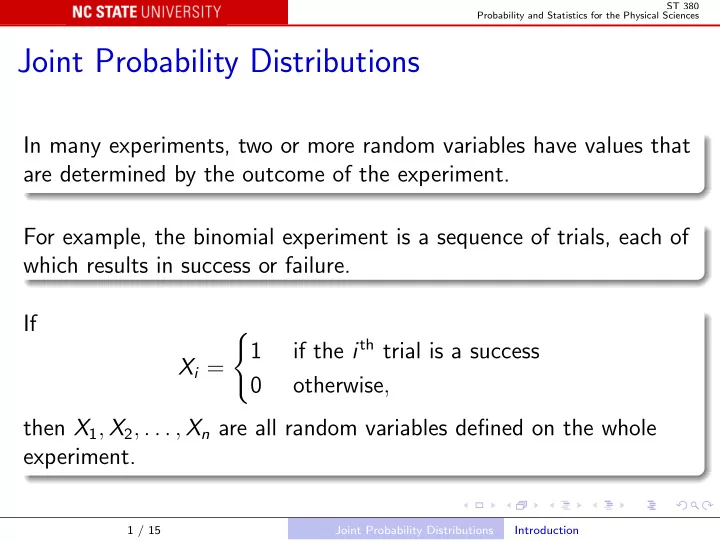
In many experiments, two or more random variables have values that are determined by the outcome of the experiment. For example, the binomial experiment is a sequence of trials, each of which results in success or failure. If Xi =

• 1

if the ith trial is a success

• therwise,

then X1, X2, . . . , Xn are all random variables defined on the whole experiment.

1 / 15 Joint Probability Distributions Introduction

ST 380 Probability and Statistics for the Physical Sciences

To calculate probabilities involving two random variables X and Y such as P(X > 0 and Y ≤ 0), we need the joint distribution of X and Y . The way we represent the joint distribution depends on whether the random variables are discrete or continuous.

2 / 15 Joint Probability Distributions Introduction

ST 380 Probability and Statistics for the Physical Sciences

Two Discrete Random Variables

If X and Y are discrete, with ranges RX and RY , respectively, the joint probability mass function is p(x, y) = P(X = x and Y = y), x ∈ RX, y ∈ RY . Then a probability like P(X > 0 and Y ≤ 0) is just

• x∈RX :x>0
• y∈RY :y≤0

p(x, y).

3 / 15 Joint Probability Distributions Two Discrete Random Variables

ST 380 Probability and Statistics for the Physical Sciences

Marginal Distribution To find the probability of an event defined only by X, we need the marginal pmf of X: pX(x) = P(X = x) =

• y∈RY

p(x, y), x ∈ RX. Similarly the marginal pmf of Y is pY (y) = P(Y = y) =

• x∈RX

p(x, y), y ∈ RY .

4 / 15 Joint Probability Distributions Two Discrete Random Variables

ST 380 Probability and Statistics for the Physical Sciences

Two Continuous Random Variables

If X and Y are continuous, the joint probability density function is a function f (x, y) that produces probabilities: P[(X, Y ) ∈ A] =

• A

f (x, y) dy dx. Then a probability like P(X > 0 and Y ≤ 0) is just ∞

−∞

f (x, y) dy dx.

5 / 15 Joint Probability Distributions Two Continuous Random Variables

ST 380 Probability and Statistics for the Physical Sciences

Marginal Distribution To find the probability of an event defined only by X, we need the marginal pdf of X: fX(x) = ∞

−∞

f (x, y) dy, −∞ < x < ∞. Similarly the marginal pdf of Y is fY (y) = ∞

−∞

f (x, y) dx, −∞ < y < ∞.

6 / 15 Joint Probability Distributions Two Continuous Random Variables

ST 380 Probability and Statistics for the Physical Sciences

Independent Random Variables

Independent Events Recall that events A and B are independent if P(A and B) = P(A)P(B). Also, events may be defined by random variables, such as A = {X ≥ 0} = {s ∈ S : X(s) ≥ 0}. We say that random variables X and Y are independent if any event defined by X is independent of every event defined by Y .

7 / 15 Joint Probability Distributions Independent Random Variables

ST 380 Probability and Statistics for the Physical Sciences

Independent Discrete Random Variables Two discrete random variables are independent if their joint pmf satisfies p(x, y) = pX(x)pY (y), x ∈ RX, y ∈ RY . Independent Continuous Random Variables Two continuous random variables are independent if their joint pdf satisfies f (x, y) = fX(x)fY (y), −∞ < x < ∞, −∞ < y < ∞. Random variables that are not independent are said to be dependent.

8 / 15 Joint Probability Distributions Independent Random Variables

ST 380 Probability and Statistics for the Physical Sciences

More Than Two Random Variables Suppose that random variables X1, X2, . . . , Xn are defined for some experiment. If they are all discrete, they have a joint pmf: p (x1, x2, . . . , xn) = P(X1 = x1, X2 = x2, . . . , Xn = xn). If they are all continuous, they have a joint pdf: P(a1 < X1 ≤ b1, . . . , an < Xn ≤ bn) = b1

a1

. . . bn

an

f (x1, . . . , xn) dxn . . . dx1.

9 / 15 Joint Probability Distributions Independent Random Variables

ST 380 Probability and Statistics for the Physical Sciences

Full Independence The random variables X1, X2, . . . , Xn are independent if their joint pmf or pdf is the product of the marginal pmfs or pdfs. Pairwise Independence Note that if X1, X2, . . . , Xn are independent, then every pair Xi and Xj are also independent. The converse is not true: pairwise independence does not, in general, imply full independence.

10 / 15 Joint Probability Distributions Independent Random Variables

ST 380 Probability and Statistics for the Physical Sciences

Conditional Distribution If X and Y are discrete random variables, then P(Y = y|X = x) = P(X = x and Y = y) P(X = x) = p(x, y) pX(x) . We write this as pY |X(y|x). If X and Y are continuous random variables, we still need to define the distribution of Y given X = x. But P(X = x) = 0, so the definition is not obvious; however, fY |X(y|x) = f (x, y) fX(x) may be shown to have the appropriate properties.

11 / 15 Joint Probability Distributions Independent Random Variables

ST 380 Probability and Statistics for the Physical Sciences

Expected Value, Covariance, and Correlation

As you might expect, for a function of several discrete random variables: E[h(x1, . . . , xn)] =

• x1

· · ·

• xn

h(x1, . . . , xn)p(x1, . . . , xn) For a function of several continuous random variables: E[h(x1, . . . , xn)] = ∞

−∞

. . . ∞

−∞

h(x1, . . . , xn)f (x1, . . . , xn) dxn . . . dx1.

12 / 15 Joint Probability Distributions Expected Value, Covariance, and Correlation

ST 380 Probability and Statistics for the Physical Sciences

Covariance Recall the variance of X: V (X) = E

• (X − µX)2

. The covariance of two random variables X and Y is Cov(X, Y ) = E [(X − µX)(Y − µY )] . Note: the covariance of X with itself is its variance.

13 / 15 Joint Probability Distributions Expected Value, Covariance, and Correlation

ST 380 Probability and Statistics for the Physical Sciences

Correlation Just as the units of V (X) are the square of the units of X, so the units of Cov(X, Y ) are the product of the units of X and Y . The corresponding dimensionless quantity is the correlation: Corr(X, Y ) = ρX,Y = Cov(X, Y ) σXσY = Cov(X, Y )

• V (X)V (Y )

.

14 / 15 Joint Probability Distributions Expected Value, Covariance, and Correlation

ST 380 Probability and Statistics for the Physical Sciences

Properties of Correlation If ac > 0, Corr(aX + b, cY + d) = Corr(X, Y ). For any X and Y , −1 ≤ Corr(X, Y ) ≤ 1. If X and Y are independent, then Corr(X, Y ) = 0, but not

• conversely. That is, Corr(X, Y ) = 0 does not in general mean that X

and Y are independent. If Corr(X, Y ) = ±1, then X and Y are exactly linearly related: Y = aX + b for some a = 0.

15 / 15 Joint Probability Distributions Expected Value, Covariance, and Correlation