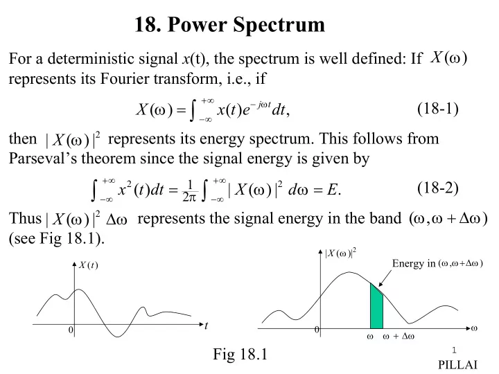
= + j t (18-1) X ( ) x t e ( ) dt , X then - PowerPoint PPT Presentation

18. Power Spectrum X ω ( ) For a deterministic signal x (t), the spectrum is well defined: If represents its Fourier transform, i.e., if = ∫ +∞ ω − ω j t (18-1) X ( ) x t e ( ) dt , −∞ X ω then represents its energy spectrum. This follows from 2 | ( ) | Parseval’s theorem since the signal energy is given by +∞ +∞ ∫ 1 ∫ = ω ω = 2 2 (18-2) x t dt ( ) | X ( ) | d E . π 2 −∞ −∞ ω ω + ∆ ω X ω ∆ ω 2 ( , ) Thus represents the signal energy in the band | ( ) | (see Fig 18.1). 2 X ω | ( )| ω ω +∆ ω Energy in ( , ) X t ( ) t ω 0 0 ω ω + ∆ ω Fig 18.1 1 PILLAI

However for stochastic processes, a direct application of (18-1) ω . generates a sequence of random variables for every Moreover, for a stochastic process, E {| X ( t ) | 2 } represents the ensemble average power (instantaneous energy) at the instant t . To obtain the spectral distribution of power versus frequency for stochastic processes, it is best to avoid infinite intervals to begin with, and start with a finite interval (– T , T ) in (18-1). Formally, partial Fourier transform of a process X ( t ) based on (– T , T ) is given by = ∫ T ω − ω j t (18-3) X ( ) X t e ( ) dt T − T so that ω 2 | X ( ) | 1 2 T ∫ = − ω j t T X t e ( ) dt (18-4) 2 T 2 T − T represents the power distribution associated with that realization based on (– T , T ). Notice that (18-4) represents a random variable for every ω , and its ensemble average gives, the average power distribution based on (– T , T ). Thus 2 PILLAI

 ω 2  | X ( ) | 1 T T ∫ ∫ − ω − ω = = j ( t t ) * P ( ) E T E X t X { ( ) ( )} t e dt dt   1 2 1 2 1 2 T 2 T 2 T − −   T T 1 T T ∫ ∫ = − ω − j ( t t ) R ( , t t e ) dt dt (18-5) 1 2 1 2 1 2 2 T − − XX T T represents the power distribution of X ( t ) based on (– T , T ). For wide sense stationary (w.s.s) processes, it is possible to further simplify = − R ( , ) t t R ( t t ) (18-5). Thus if X ( t ) is assumed to be w.s.s, then 1 2 1 2 XX XX and (18-5) simplifies to 1 T T ∫ ∫ ω = − − ω − j ( t t ) P ( ) R ( t t e ) dt dt . 1 2 1 2 1 2 T 2 T − − XX T T τ = − t t Let and proceeding as in (14-24), we get 1 2 1 2 T ∫ − ωτ ω = τ − τ τ j P ( ) R ( ) e (2 T | |) d T 2 T − XX 2 T 2 T ∫ − ωτ τ = τ − | | τ ≥ j (18-6) R ( ) e (1 ) d 0 2 T − XX 2 T to be the power distribution of the w.s.s. process X ( t ) based on 3 T → ∞ (– T , T ). Finally letting in (18-6), we obtain PILLAI

+∞ ∫ ω = ω = τ − ωτ τ ≥ j (18-7) S ( ) lim P ( ) R ( ) e d 0 XX T −∞ XX →∞ T to be the power spectral density of the w.s.s process X ( t ). Notice that ω ←→ ⋅ ω ≥ F T R ( ) S ( ) 0. (18-8) XX XX i.e., the autocorrelation function and the power spectrum of a w.s.s Process form a Fourier transform pair, a relation known as the Wiener-Khinchin Theorem . From (18-8), the inverse formula gives +∞ 1 ∫ τ = ω ωτ ω j R ( ) S ( ) e d (18-9) π 2 XX −∞ XX τ = and in particular for we get 0, +∞ 1 ∫ ω ω = = = 2 S ( ) d R (0) E {| X t ( ) | } P , the total power. π 2 −∞ XX XX (18-10) ω From (18-10), the area under represents the total power of the S ( ) XX ω process X ( t ), and hence truly represents the power S ( ) XX 4 spectrum. (Fig 18.2). PILLAI

ω S ( ) ω ∆ ω S ( ) represents the power XX XX ω ω + ∆ ω in the band ( , ) ω ω ω + ∆ ω 0 Fig 18.2 The nonnegative-definiteness property of the autocorrelation function in (14-8) translates into the “nonnegative” property for its Fourier transform (power spectrum), since from (14-8) and (18-9) n n n n +∞ ∑∑ ∑∑ ω − 1 ∫ j ( t t ) − = ω ω * * a a R ( t t ) a a S ( ) e d i j π 2 i j i j i j XX −∞ XX = = = = i 1 j 1 i 1 j 1 2 +∞ ∑ 1 n ∫ ω = ω j t ω ≥ S ( ) a e d 0. (18-11) i π 2 = i i 1 −∞ XX From (18-11), it follows that τ ⇔ ω ≥ R ( ) nonnegative - definite S ( ) 0. (18-12) XX XX 5 PILLAI

If X ( t ) is a real w.s.s process, then so that τ − τ R ( ) = R ( ) XX XX +∞ ∫ − ωτ ω = τ τ j S ( ) R ( ) e d XX −∞ XX +∞ ∫ = τ ωτ τ R ( )cos d −∞ XX ∞ ∫ = τ ωτ τ = − ω ≥ (18-13) 2 R ( )cos d S ( ) 0 XX XX 0 so that the power spectrum is an even function, (in addition to being real and nonnegative). 6 PILLAI

Power Spectra and Linear Systems If a w.s.s process X ( t ) with autocorrelation h ( t ) τ ↔ τ ≥ function is X ( t ) Y ( t ) R ( ) S ( ) 0 XX XX applied to a linear system with impulse Fig 18.3 response h ( t ), then the cross correlation τ R ( ) function and the output autocorrelation function are τ R ( ) XY YY given by (14-40)-(14-41). From there τ = τ ∗ − τ τ = τ ∗ − τ ∗ τ * * R ( ) R ( ) h ( ), R ( ) R ( ) h ( ) h ( ). (18-14) XY XX YY XX But if (18-15) ↔ ω ↔ ω f t ( ) ( ), ( ) F g t ( ) G Then ∗ ↔ ω ω f t ( ) g t ( ) ( ) ( ) F G (18-16) since +∞ ∫ ∗ = ∗ − ω j t { ( ) f t g t ( )} f t ( ) g t e ( ) dt F 7 −∞ PILLAI

{ } +∞ +∞ ∫ ∫ ∗ τ − τ τ − ω j t { ( ) f t g t ( )}= f ( ) ( g t ) d e dt F −∞ −∞ +∞ +∞ ∫ ∫ τ − ωτ τ − τ − ω − τ − τ j j ( t ) = f ( ) e d g t ( ) e d t ( ) −∞ −∞ ω ω (18-17) = ( ) ( ). F G Using (18-15)-(18-17) in (18-14) we get ω = ω ∗ − τ = ω ω (18-18) * * S ( ) { R ( ) h ( )} S ( ) H ( ) F XY XX XX since ( ) * +∞ +∞ ∫ ∫ − τ − ωτ τ = − ω = ω * j j t * h ( ) e d h t e ( ) dt H ( ), −∞ −∞ where = ∫ +∞ (18-19) ω − ω j t H ( ) h t e ( ) dt −∞ represents the transfer function of the system, and ω = τ = ω ω S ( ) F { R ( )} S ( ) H ( ) YY YY XY = ω ω 2 S ( ) | H ( ) | . (18-20) 8 XX PILLAI

From (18-18), the cross spectrum need not be real or nonnegative; However the output power spectrum is real and nonnegative and is related to the input spectrum and the system transfer function as in (18-20). Eq. (18-20) can be used for system identification as well. W.S.S White Noise Process : If W ( t ) is a w.s.s white noise process, then from (14-43) τ = δ τ ⇒ ω = R ( ) q ( ) S ( ) q . (18-21) WW WW Thus the spectrum of a white noise process is flat, thus justifying its name. Notice that a white noise process is unrealizable since its total power is indeterminate. From (18-20), if the input to an unknown system in Fig 18.3 is a white noise process, then the output spectrum is given by ω = ω 2 (18-22) S ( ) q H | ( ) | YY Notice that the output spectrum captures the system transfer function characteristics entirely, and for rational systems Eq (18-22) may be used to determine the pole/zero locations of the underlying system. 9 PILLAI

Example 18.1 : A w.s.s white noise process W ( t ) is passed through a low pass filter (LPF) with bandwidth B /2. Find the autocorrelation function of the output process. Solution: Let X ( t ) represent the output of the LPF. Then from (18-22) ω ≤  q , | | B / 2 ω = ω =  2 S ( ) q H | ( ) | . (18-23) ω > 0, | | B / 2 XX  Inverse transform of gives the output autocorrelation function ω S ( ) XX to be / 2 B ωτ B / 2 ωτ τ = ω ω = ω j j R ( ) S ( ) e d q e d ∫ ∫ − − B / 2 B / 2 XX XX τ sin( B / 2) = = τ qB qB sinc( B / 2) (18-24) τ ( B / 2) τ R ( ) XX 2 qB H ω | ( )| 1 τ ω − B / 2 B / 2 (a) LPF (b) 10 Fig. 18.4 PILLAI

Eq (18-23) represents colored noise spectrum and (18-24) its autocorrelation function (see Fig 18.4). Example 18.2: Let 1 + t T ∫ = τ τ (18-25) Y t ( ) X ( ) d − t T 2 T represent a “smoothing” operation using a moving window on the input process X ( t ). Find the spectrum of the output Y ( t ) in term of that of X ( t ). h t ( ) 1 / 2 T Solution : If we define an LTI system with impulse response h ( t ) as in Fig 18.5, t − T T then in term of h ( t ), Eq (18-25) reduces to Fig 18.5 +∞ ∫ = − τ τ τ = ∗ Y t ( ) h t ( ) X ( ) d h t ( ) X t ( ) (18-26) −∞ so that ω = ω ω (18-27) 2 S ( ) S ( ) | H ( ) | . YY XX Here + T ∫ ω = − ω = ω j t H ( ) e dt sinc( T ) 1 (18-28) 11 2 T − T PILLAI