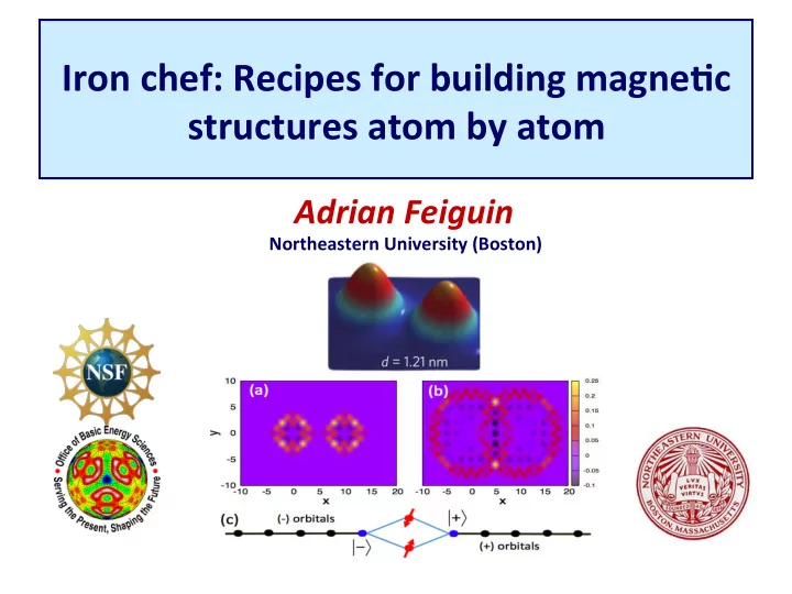
Iron chef: Recipes for building magne6c structures atom by - - PowerPoint PPT Presentation

SLIDE 1

Iron ¡chef: ¡Recipes ¡for ¡building ¡magne6c ¡ structures ¡atom ¡by ¡atom ¡

Adrian ¡Feiguin ¡

Northeastern ¡University ¡(Boston) ¡

SLIDE 2

Northeastern ¡University ¡

Boston ¡

SLIDE 3

Assistant ¡chefs ¡

Carlos ¡Busser ¡ Andrew ¡Allerdt ¡ References: ¡ A.Allerdt, ¡C. ¡A. ¡Büsser, ¡S. ¡Das ¡Sarma, ¡A. ¡E. ¡Feiguin ¡(in ¡prepara<on). ¡ ¡A. ¡Allerdt, ¡C. ¡A. ¡Büsser, ¡ ¡G. ¡B. ¡Mar<ns, ¡and ¡A. ¡E. ¡Feiguin, ¡Phys. ¡Rev. ¡B ¡91, ¡085101 ¡(2015). ¡ ¡ ¡

• C. ¡A. ¡Büsser, ¡ ¡G. ¡B. ¡Mar<ns, ¡and ¡A. ¡E. ¡Feiguin, ¡Phys. ¡Rev. ¡B ¡88, ¡245113 ¡(2013). ¡ ¡

SLIDE 4

Mo6va6on ¡I: ¡Permanent ¡magnets ¡are ¡of ¡ strategic ¡importance ¡for ¡modern ¡technology ¡

4 Computer and

• ffice

automation

• Computer hard drives
• CD-ROM spindle motors and

pick-up motors Consumer electronics

• cameras
• speakers
• cell phones

Automotive & transportation

• starter motors
• electric steering
• sensors
• instrumentation gauges

Medical industry

• magnetic resonance imaging

equipment

• surgical tools
• medical implants

Factory automation

• magnetic couplings
• servo motors
• generators
• magnetic bearings

Alternative energy

• hybrid/electric vehicles
• wind power systems
• power generation systems
• energy storage systems

Appliances & systems

• portable power tools
• household appliance motors
• scales
• air conditioners

Military

• weapons systems
• vehicles, watercraft, avionics
• communications systems, radar

satellites

Energy Conversion Data & Electronics

Courtesy of Luke G. Marshall: Table adapted from: Lewis, L. H. & Jiménez-Villacorta, F. “Perspectives on Permanent Magnetic Materials for Energy Conversion and Power Generation.” Metall. Mater. Trans. A 44, 2–20 (2012). Systems information from USMMA RE-Weapons Systems DoD Supply Chain Assessment, 10/07/2010: http://bit.ly/1THp1uM

SLIDE 5

RE-­‑elements ¡supply ¡chain ¡

• M. Humphries. “Rare Earth Elements: The Global Supply Chain.” Congressional Research Service 7-5700, R41347, 2011.

5

SLIDE 6

RE-­‑elements ¡supply ¡chain ¡ An ¡strategic ¡priority ¡area ¡

Clean energy TeChnologies and

solar Cells Wind Turbines Vehicles lightjng

MaTerial

PV fjlms Magnets Magnets Batueries Phosphors lanthanum

• Cerium
• Praseodymium
• neodymium
• samarium
• europium
• Terbium
• dysprosium
• yturium
• indium
• gallium
• Tellurium
• Cobalt
• lithium
• Figure 1. Short-Term (0–5 years)

Criticality Matrix

• Critjcal Near Critjcal Not Critjcal

Figure 2. Medium-Term (5–15 years) Criticality Matrix

• Critjcal Near Critjcal Not Critjcal

DOE ¡Report, ¡2010 ¡(see ¡also ¡DOD ¡reports) ¡

SLIDE 7

(Possible ¡and ¡likely) ¡Solu6on: ¡ Asteroid ¡Mining ¡

hNp://www.planetaryresources.com ¡

Asteroid ¡Redirect ¡Mission ¡(NASA ¡and ¡Planetary ¡Resources) ¡

SLIDE 8

Asteroid ¡mining ¡

hNp://www.planetaryresources.com ¡

SLIDE 9

Mo6va6on ¡II: ¡“Spintronics” ¡

• Informa<on ¡is ¡stored ¡into ¡spin ¡as ¡one ¡of ¡two ¡possible ¡
• rienta<ons ¡
• Spin ¡life<me ¡is ¡rela<vely ¡long, ¡on ¡the ¡order ¡of ¡nanoseconds ¡ ¡
• Spin ¡currents ¡can ¡be ¡manipulated ¡
• Spin ¡devices ¡may ¡combine ¡logic ¡and ¡storage ¡func<onality ¡

elimina<ng ¡the ¡need ¡for ¡separate ¡components ¡

• Magne<c ¡storage ¡is ¡nonvola<le ¡
• Binary ¡spin ¡polariza<on ¡offers ¡the ¡possibility ¡of ¡ ¡

applica<ons ¡as ¡qubits ¡(quantum ¡“spins ¡transistors”) ¡in ¡ quantum ¡computers ¡

• High ¡speed, ¡low ¡power ¡consump<on ¡
• Atomic ¡scale ¡devices ¡

SLIDE 10

Mo6va6on ¡III: ¡fundamental ¡physics ¡and ¡ exo6c ¡states ¡of ¡maIer ¡

Topological ¡states ¡ ¡ Spin ¡liquids ¡ Spin ¡glasses ¡ Many-­‑body ¡localiza<on ¡

SLIDE 11

Classical ¡magne6sm ¡(or ¡lack ¡thereof) ¡

The ¡Bohr-­‑van ¡Leeuwen ¡theorem ¡ ¡

F = qv × B Perpendicular ¡to ¡velocity ¡ F⋅dl

∫

= F⋅vdt = q (v × B)⋅vdt =

∫ ∫

No ¡work ¡

No ¡work ¡= ¡no ¡change ¡in ¡energy ¡= ¡no ¡magne<za<on!!! ¡

R v B

Simple ¡proof: ¡

H = pi +eA(r

i)

[ ]

2

2m

i

∑

+other terms

Z = dridpi exp −βH({ri,pi})

[ ]

i

∏ ∫

M = − ∂F ∂B " # $ % & '

T,V

= − 1 β ∂ logZ ∂B " # $ % & '

T,V

= 0 Actual ¡proof: ¡ The ¡vector ¡poten<als ¡can ¡be ¡“gauged ¡out”, ¡the ¡integral ¡is ¡independent ¡of ¡B ¡

!!! ¡

The ¡Bohr-­‑van ¡Leeuwen ¡theorem ¡shows ¡that ¡magne<sm ¡cannot ¡be ¡accounted ¡for ¡

• classically. ¡In ¡par<cular, ¡it ¡also ¡rules ¡out ¡classical ¡ferromagne<sm, ¡paramagne<sm, ¡

and ¡diamagne<sm ¡(In ¡equilibrium!). ¡

SLIDE 12

Magne6sm ¡is ¡a ¡quantum ¡ phenomenon! ¡

Main ¡contribu6on ¡for ¡free ¡atoms: ¡

• ¡ ¡ ¡ ¡ ¡spins ¡of ¡electrons ¡
• ¡ ¡ ¡ ¡ ¡orbital ¡angular ¡momenta ¡of ¡electrons ¡
• ¡ ¡ ¡ ¡ ¡Induced ¡orbital ¡moments

Electronic structure Moment H: 1s M ∼ S He: 1s2 M = 0 unfilled shell M ≠ 0 All filled shells M = 0 AFM ¡ interac<ons ¡ FM ¡ interac<ons ¡

SLIDE 13

Various ¡types ¡of ¡magne6sm ¡

Source: ¡www.boundless.com ¡

Magne<sm ¡in ¡the ¡solid ¡state ¡is ¡much ¡rarer ¡than ¡in ¡gases, ¡since ¡in ¡gases ¡atoms ¡ preserve ¡their ¡par<ally ¡filled ¡shells ¡ ¡

SLIDE 14

Source: ¡www.boundless.com ¡ Colors ¡represent ¡s, ¡i, ¡d, ¡and ¡f ¡blocks ¡

Solu6on: ¡dope ¡with ¡Rare ¡Earths ¡and ¡ Transi6on ¡metals ¡

SLIDE 15

Hund’s Rules

Hund’s rule ( L-S coupling scheme ): Outer shell electrons of an atom in its ground state should assume

• 1. Maximum value of S allowed by exclusion principle.
• 2. Maximum value of L compatible with (1).
• 3. J = | L−S | for less than half-filled shells.

J = L + S for more than half-filled shells. Causes:

• 1. Parallel spins have lower Coulomb energy.
• 2. e’s meet less frequently if orbiting in same direction (parallel Ls).
• 3. Spin orbit coupling lowers energy for L⋅S < 0.

For filled shells, spin orbit couplings do not change order of levels. Mn2+: 3d 5 (1) → S = 5/2 exclusion principle → L = 2+1+0−1−2 = 0 Ce3+: 4 f 1 L = 3, S = ½ (3) → J = | 3− ½ | = 5/2 Pr3+: 4 f 2 (1) → S = 1 (2) → L = 3+2 = 5 (3) → J = | 5− 1 | = 4

2 5/2

F

3 4

H

SLIDE 16

Iron ¡Group ¡Ions

L = 0 From Kittel’s “Solid State Physics” In ¡these ¡ions, ¡the ¡magneton ¡numbers ¡agree ¡well ¡with ¡the ¡spin ¡predic<on, ¡as ¡ though ¡the ¡orbital ¡moment ¡were ¡not ¡present ¡(it’s ¡said ¡to ¡be ¡“quenched”) ¡ ¡ ¡

SLIDE 17

(Some) ¡Types ¡of ¡magne6sm ¡

Paramagne<sm ¡ Ferromagne<sm ¡ An<-­‑Ferromagne<sm ¡ Ferrimagne<sm ¡ An<-­‑Ferromagne<c ¡interac<ons ¡can ¡ yield ¡counter-­‑intui<ve ¡states ¡of ¡ purely ¡quantum ¡origin, ¡such ¡as ¡ “spin-­‑liquids” ¡

SLIDE 18

The ¡power ¡of ¡STM ¡ ¡

Andreas ¡Heinrich, ¡Physics ¡Today ¡(March ¡2015) ¡

• STM ¡provides ¡a ¡tool ¡for ¡construc<ng ¡magne<c ¡structures ¡atom ¡by ¡atom ¡
• STM-­‑based ¡spectroscopies ¡can ¡probe ¡magne<c ¡interac<ons ¡with ¡atomic ¡

resolu<on, ¡such ¡as: ¡

• Interplay ¡between ¡a ¡local ¡spin ¡and ¡its ¡local ¡environment ¡
• accessing ¡mul<-­‑spin ¡systems ¡and ¡probing ¡for ¡many-­‑body ¡effects ¡

Gerd Binnig and Heinrich Rohrer 1986 Nobel Price

SLIDE 19

Coupling ¡between ¡spins ¡and ¡their ¡ environment ¡

In ¡some ¡cases, ¡such ¡as ¡in ¡quantum ¡informa<on ¡processing, ¡spins ¡are ¡extremely ¡sensi<ve ¡to ¡ decoherence, ¡a ¡randomiza<on ¡of ¡the ¡spin ¡state ¡caused ¡by ¡entanglement ¡with ¡the ¡environment ¡ ¡

environment is in

In ¡other ¡circumstances, ¡this ¡coupling ¡is ¡crucial, ¡and ¡can ¡be ¡used ¡to ¡engineer ¡magne<c ¡structures ¡ with ¡arbitrary ¡interac<ons ¡

SLIDE 20

Atomic ¡scale ¡magne6c ¡structures ¡

• S. Loth et al

Science (2013)

Ladders ¡and ¡magne<c ¡clusters ¡ Spin ¡chains ¡ Frustra<on ¡

Spinelli et al

• Nat. Mat. (2014)

B = -0.625 T

1 nm 0.5 Å

Khajetoorians et al

• Nat. Phys. (2012)

Khajetoorians et al Science (2011)

Skyrmions ¡

Von Bergmann

• Nano. Lett. (2015)

Khajetoorians et al Science (2011)

Magne<c ¡devices ¡

SLIDE 21

From ¡single ¡atoms ¡to ¡magne6c ¡structures ¡

Isolated ¡single ¡ atoms ¡ Insula<ng ¡substrate ¡ Metallic ¡substrate ¡ Single ¡atom ¡ proper<es ¡ Coopera<ve/many-­‑body ¡ correla<on ¡effects ¡ Kondo ¡ effect ¡ Distance ¡ dependent ¡ interac<ons ¡ (RKKY) ¡ Magne<c ¡ nano-­‑ structures ¡

SLIDE 22

The ¡single-­‑impurity ¡(Kondo) ¡problem ¡

Lagce ¡details ¡and ¡dimensionality ¡do ¡not ¡play ¡a ¡relevant ¡role ¡in ¡the ¡**universal** ¡ physics ¡of ¡the ¡single ¡impurity, ¡unless: ¡

• There ¡is ¡a ¡gap ¡(band ¡insulators) ¡
• a ¡pseudogap ¡(graphene) ¡
• a ¡“patological” ¡DOS ¡(van ¡Hove ¡singularity) ¡
• Small ¡system ¡(Kondo ¡box) ¡

Wilson: ¡Regardless ¡of ¡the ¡dimensionality, ¡the ¡Kondo ¡problem ¡is ¡essen<ally ¡one-­‑ dimensional ¡. ¡ It ¡can ¡be ¡solved ¡with ¡Numerical ¡Renormaliza<on ¡Group ¡(Wilson, ¡Krishnamurthy, ¡ Wilkins), ¡or ¡Bethe ¡Ansatz ¡(Tsvelik, ¡Andrei). ¡

Metal surface Magnetic atom

SLIDE 23

A ¡single ¡magne6c ¡impurity: ¡The ¡ Kondo ¡problem ¡

Yong-­‑Hui ¡Zhang, ¡Nature ¡Comm. ¡(2013) ¡

SLIDE 24

Wilson’s ¡NRG ¡approach ¡

808

Kenneth

• G. Wilson: The renormalization

group

states correspond

(roughly)

to spherical

layers surrounding the imp urity, as shown in

• Fig. 13. That

is, the wave function for the second state of the Kondo basis is nonzero (except for small tails)

• nly

in the first spherical shell marked g 1 in Fig. 13, with width

• Al. Here
• A. is a pa-

rameter &1; it can be chosen arbitrarily. See below. For accidental reasons the width

• f the first layer

is denoted

A& rather

than

• A. The third

state

is predominantly con- tained in shell g2, etc. The shells increase in width; and correspondingly the momentum spread of succeeding

states decreases.

All wave

functions

in the Kondo

basis are de- fined so that their average momentum is the Fermi mo- mentum. As n increases the nth

state

is concentrated closer and closer to the

Fermi surface; thus the energy scale for these states decreases being

A "I' for

the nth state.

• FIG. 13.

Onion-like spherical shells giving the location of successive wave functions in the Kondo basis. The size of the smallest (inner) shell is a few Angstrom units.

energy

• scale. Figure

12 with

• nly

two energy levels

per scale is thus an oversimplification. Here and throughout the Kondo calculations the

em- phasis is

• n

properties

• f the

conduction band rather than the impurity

• itself. One might

think that the peculiar nature

• f the Kondo problem

is due to the magnetic im-

purity, not the conduction band. The importance

• f the

impurity is simple: it forces one to study the conduction band as a many-electrori

• system. The cause of this is spin-

fiip

scat tering

• 6 the

impurity, which is possible

• nly

when

the impurity

is magnetic

(i.e., has a spin). Suppose

two electrons,

both

with spin up, try to spin-Rip

scatter

from a spin-down impurity.

The first electron can spin-Aip scatter, but the result is to leave the impurity

with spin up.

The second

electron

now cannot spin-Rip

scatter

because this

would

violate

spin

conservation. Thus

• ne

cannot treat the electrons

• f the conduction

band independently:

• ne must

treat

the conduction band as a many electron system. Inevitably, as a many-electron system, the con- duction band has the energy

level structure

indicated

in

• Fig. 12, with

each energy scale corresponding to a dif- ferent set of electrons. The normal description

• f individual

electrons

in

the conduction band

is in terms of plane wave or Bloch wave

states. This

description is poorly

• suited. to

the Kondo calculations. The trouble is that there are too many plane wave states with almost the same energy (due to the plane wave states being close to a continuum for a sample

• f macroscopic

size). For the Kondo calculation

it was

necessary to define a new basis of states in the conduction band which emphasizes those states with the largest direct

• r

indirect interaction with the impurity. The states chosen are closer to the localized Wannier states than the Bloch waves. The first state is (at least roughly) a Wannier

state localized about the impurity,

as localized as possible

while still being in the

conduction

band. The remaining In

this basis, electron states are neglected where the electron is far away from the impurity in position space and far away from the Fermi surface in momentum

space. The motivation for this

is as follows.

The

• nly

reason for considering

states far away

from the impurity

at all

is that at very low temperatures

• nly electrons

very close to the Fermi surface are thermally

• excited. Being close to

the Fermi surface in momentum space means the elec- trons have very broad wave functions in position space. At

low

temperatures the impurity interacts with these states near the Fermi surface; hence they must be included

in the basis.

It is possible

to add more states to the Kondo basis to make it complete. This is explained later

in this Section.

It turns

• ut to be a good approximation

(for static ther- modynamic calculations) to neglect these extra states. See later in this Section for more discussion. The conduction band is now approximated by an infinite set of discrete electron

levels (called

the "Kondo basis") arranged much like layers

• f an
• nion

surrounding the impurity.

The energy scale on the nth level is of order A "I'. The heart

• f the Kondo calculation

is a solution

• f the

Kondo Hamiltonian

in the Kondo basis using numerical

methods. This proceeds

in

steps. First

• ne

solves the impurity coupled

to the first Kondo state

(in the num- bering

• f Sec. VIII this is the 0th step). The next step is

to add the second layer

• f the onion,

namely the terms involving the second Kondo state, and solve the combined coupling

• f the

first and second conduction band

states to the impurity. Then one adds the third state, then the

fourth

state, and so forth. This corresponds to solving for

the eigenvalues

at successively

smaller and smaller energy scales in Fig. 12.

Beyond the first

few steps

this calculation cannot be done exactly: there are too many

• states. To be precise,

there are 2'"+' states in the nth step; when n is about 5

• r higher

this number is too large for an exact calculation. Therefore, an approximate method is used which generates

• nly

the lowest energy

levels

at each step;

in practice this means calculating

about the first 1000 energy levels. Note that for large n, say n = 100, the first 1000 energy

levels are a negligible

fraction of the total number

• f levels

(2"' for n = 100).

• Rev. Mod. Phys. , Vol. 4?, No. 4, October 1S?5
• Change ¡of ¡basis: ¡Pick ¡orthogonal ¡discre<zed ¡shells ¡around ¡the ¡impurity ¡with ¡

spherical ¡(s-­‑wave ¡symmetry ¡-­‑-­‑All ¡other ¡symmetry ¡channels ¡are ¡ignored, ¡it ¡can ¡be ¡ shown ¡that ¡they ¡don’t ¡play ¡a ¡role) ¡

• The ¡farther ¡the ¡state, ¡the ¡closer ¡it ¡is ¡to ¡the ¡Fermi ¡energy ¡
• A ¡“lambda” ¡or ¡logarithmic ¡discre<za<on ¡of ¡the ¡spectrum ¡increases ¡resolu<on ¡

around ¡the ¡Fermi ¡energy ¡and ¡ ¡enables ¡an ¡RG ¡analysis ¡ ¡

• −1
• −3

−2

• −1

−3

• −2

...

• ()
• −1

−1 1 1

()

• t

t

V

t 0

1 2 1 2 3

b) a) c)

Wilson’s ¡RMP(75), ¡Bulla, ¡Cos<, ¡Pruschke, ¡RMP(08). ¡

SLIDE 25

Introducing ¡the ¡laUce ¡

• C. ¡A. ¡Busser, ¡G. ¡B. ¡Mar<ns, ¡and ¡A. ¡E. ¡Feiguin, ¡Phys. ¡Rev. ¡B ¡ ¡88, ¡245113 ¡(2013). ¡
• R. ¡Haydock, ¡V. ¡Heine, ¡and ¡M. ¡Kelly, ¡Journal ¡of ¡Physics ¡C: ¡Solid ¡State ¡Physics ¡5, ¡2845 ¡(1972). ¡

¡ ¡

• 1. ¡Choose ¡the ¡seed: ¡
• 2. ¡Lanczos ¡Itera<on: ¡

Ψ 1 = H Ψ0 − a0 Ψ0

Ψ i+1 = H Ψi −ai Ψi −bi

2 Ψi−1

Ψ0 = c†

r

0 0

ai = Ψi H Ψi Ψi Ψi bi = Ψi Ψi Ψi−1 Ψi−1

We ¡choose ¡a ¡basis ¡of ¡concentric ¡orbitals ¡that ¡expand ¡radially ¡from ¡the ¡impurity ¡a ¡la ¡

• Wilson. ¡The ¡are ¡generated ¡by ¡the ¡ac<on ¡of ¡the ¡non-­‑interac<ng ¡hopping ¡terms. ¡

SLIDE 26

Lanczos ¡Orbitals ¡

n=0 ¡ seed ¡ n=1 ¡ n=2 ¡ n=3 ¡ n=4 ¡ n=5 ¡ n=6 ¡ n=7 ¡ n=8 ¡

SLIDE 27

The ¡equivalent ¡chain ¡

Hband= a0 b

1

b

1

a1 b2 b2 a2 b3 b3 a3 ! ! ! ! " # # # # # # # $ % & & & & & & &

Hband = (bic†

ici−1 + h.c.)+

aini

i=0 N

∑

i=1 N

∑

Same ¡as ¡Wilson’s ¡approach, ¡the ¡Hamiltonian ¡now ¡is ¡in ¡Tri-­‑Diagonal ¡Form: ¡

Can ¡study ¡ systems ¡with ¡ Ld ¡sites, ¡ keeping ¡only ¡ ~O(L) ¡orbitals! ¡ ¡

SLIDE 28

Example: ¡Square ¡LaUce ¡

LDOS ¡

New ¡“Hopping” ¡

ρ0(ω) = − 1 π lim

η→0 ImG0(ω +iη)

SLIDE 29

Cubic ¡ 1D ¡chain ¡ Honeycomb ¡ Triangular ¡

SLIDE 30

The ¡effec6ve ¡Hamiltonian ¡

• The ¡impurity ¡is ¡connected ¡to ¡the ¡first ¡site ¡of ¡the ¡chain ¡(which ¡remains ¡in ¡a ¡real ¡space ¡

representa<on), ¡and ¡the ¡many-­‑body ¡terms ¡only ¡act ¡on ¡that ¡link. ¡

• The ¡impurity ¡(rigorously) ¡only ¡couples ¡to ¡the ¡“s-­‑wave” ¡channel. ¡
• The ¡effec<ve ¡one-­‑dimensional ¡system ¡can ¡be ¡effec<vely ¡solved ¡with ¡DMRG. ¡

Observa6ons: ¡

• The ¡entanglement ¡in ¡free ¡fermionic ¡systems ¡can ¡be ¡understood ¡in ¡terms ¡of ¡the ¡

number ¡of ¡channels ¡<mes ¡the ¡entanglement ¡of ¡a ¡1d ¡chain. ¡

• All ¡the ¡terms ¡in ¡the ¡“s-­‑wave” ¡Hamiltonian ¡have ¡the ¡same ¡sign. ¡
• The ¡other ¡channels ¡with ¡different ¡symmetry ¡will ¡form ¡their ¡own ¡chains ¡and ¡will ¡not ¡

couple ¡to ¡the ¡impurity. ¡

• Many ¡states ¡in ¡the ¡density ¡of ¡states ¡(an ¡exponen6al ¡number) ¡**do ¡not** ¡

contribute ¡to ¡the ¡physics!!! ¡

SLIDE 31

Finite ¡size ¡effects ¡

• ­‑

In ¡finite ¡systems, ¡when ¡orbitals ¡reach ¡the ¡ boundary, ¡they ¡“bounce ¡back” ¡and ¡retrace ¡ their ¡path. ¡ ¡ ¡

• ­‑

Unless ¡the ¡lagce ¡has ¡the ¡same ¡symmetry ¡of ¡ the ¡orbitals, ¡the ¡channels ¡will ¡couple ¡at ¡the ¡

• boundary. ¡
• ­‑

Typically, ¡one ¡considers ¡“infinite ¡system/ ¡ thermodynamic ¡ ¡boundary ¡condi<ons”, ¡ where ¡the ¡orbitals ¡expand ¡indefinitely ¡ (same ¡as ¡Wilson’s ¡RG) ¡

SLIDE 32

(Some) ¡Outstanding ¡issues ¡in ¡mul6-­‑ impurity ¡problems ¡

• Non-­‑perturba<ve ¡effects ¡and ¡compe<<on ¡between ¡Kondo ¡and ¡RKKY ¡

interac<ons. ¡

• Direc<onality ¡of ¡the ¡RKKY ¡interac<on. ¡
• Ferromagne<sm. ¡
• Underscreening ¡effects. ¡ ¡
• Surface ¡and ¡(chiral) ¡edge ¡states. ¡
• Nozieres’s ¡exhaus<on ¡problem ¡and ¡fate ¡of ¡the ¡Kondo ¡cloud. ¡
• Superconduc<vity ¡and ¡Shiba ¡states. ¡

Khajetoorians, ¡A. ¡A., ¡Wiebe, ¡J., ¡Chilian, ¡ B., ¡Lounis, ¡S., ¡Blügel, ¡S., ¡Wiesendanger, ¡ R.,Nature. ¡8, ¡497-­‑503. ¡(2012) ¡ ¡ Wahlström, ¡E.,Ekvall, ¡I ¡ Olin, ¡H., ¡Walld, ¡L. ¡Appl. ¡

• Phys. ¡A ¡66, ¡S1107-­‑S1110 ¡

(1998) ¡ Prusser ¡et ¡al, ¡Nature ¡Communica<ons ¡5, ¡5417 ¡(2014) ¡ ¡

SLIDE 33

Two-­‑impurity ¡problem ¡

• 1. Choose ¡Seeds: ¡

¡

• 2. Block ¡Lanzcos1 ¡Itera<on: ¡

α0 = c†

r

1 0

β0 = c†

r2 0

α1 = H α0 − a0

αα α0 − a0 αβ β0

β1 = H β0 − a0

ββ α0 − a0 βα β0

λi+1 = H λi − ai

λγ γi γ

∑

− bi

λγ γi−1 γ

∑

R=7 ¡ R=6 ¡

• J. ¡K. ¡Cullum ¡and ¡R. ¡A. ¡Willoughby, ¡Lanczos ¡Algorithms ¡for ¡ ¡Large ¡Symmetric ¡Eigenvalue ¡

Computa=ons: ¡Vol. ¡1: ¡Theory ¡ ¡(SIAM, ¡Philadelphia, ¡2002), ¡Vol. ¡41. ¡ ¡ See ¡also ¡T. ¡Shirakawa, ¡S. ¡Yunoki, ¡PRB ¡(14) ¡

SLIDE 34

Hband= A0 B

1

B

1

A

1

B2 B2 A2 B3 B3 A3 ! ! ! ! " # # # # # # # $ % & & & & & & &

Am, Bm = n×n Matrices. ¡

n ¡= ¡# ¡of ¡‘seeds’ ¡or ¡impuri<es. ¡

See ¡also: ¡Phys. ¡Rev. ¡B ¡90, ¡195109 ¡(14). ¡Tomonori ¡Shirakawa ¡and ¡Seiji ¡Yunoki ¡ ¡

Block ¡Tri-­‑Diagonal ¡Form: ¡

SLIDE 35

Mapping ¡to ¡Chains ¡( ¡Two ¡impuri6es) ¡

• 1. Choose ¡symmetric ¡and ¡an<-­‑symmetric ¡seeds: ¡

¡ ¡

• 2. Iterate ¡the ¡same ¡as ¡the ¡single ¡impurity ¡case ¡for ¡each ¡seed. ¡

+ =

1 2 c† 1 +c2 †

( ) 0 =

1 2 1 + 2

( )

− =

1 2 c† 1 −c2 †

( ) 0 =

1 2 1 − 2

( )

SLIDE 36

Two-­‑impurity ¡Kondo ¡problem ¡

H = Hband + JK ! S1 ⋅ ! sr

1 +

! S2 ⋅ ! sr

2

( )

Auer ¡rota<ng ¡to ¡the ¡new ¡basis ¡: ¡ Iden<cal ¡to ¡the ¡Hamiltonian ¡considered ¡in ¡NRG ¡and ¡theore<cal ¡ calcula<ons, ¡but ¡in ¡“real ¡space” ¡(See ¡work ¡by ¡Wilkins, ¡Jones, ¡Varma, ¡ Affleck, ¡Ludwig, ¡etc) ¡

SLIDE 37

Our ¡conven6onal ¡understanding ¡of ¡ the ¡RKKY ¡interac6on ¡

Doniach ¡(1977) ¡

T JK

TK ∝exp − 1 JD(EF) # $ % & ' ( TRKKY ∝ J 2D(EF)

RKKY Kondo Free moments

JRKKY = J 2χ(R)

• Con<nuum ¡Model ¡
• Uniform ¡Electron ¡Gas ¡
• Quadra<c ¡Dispersion ¡

χ(R) ~ sin(2k f R+ πd

2 )

Rd

SLIDE 38

χ(r

1,r 2) = 2Re

r

1 n

n r

2

r

2 m

m r

1

En − Em

En>E f >Em

∑

Lindhard ¡func6on ¡on ¡the ¡laUce ¡

Lindhard ¡func<on: ¡ (Free ¡electron ¡suscep<bility) ¡

χ(r

i,rj) = − 1

2π Im dEG+ r

i,rj,E

( )G− r

i,rj,E

( )

−∞ ∞

∫

half-­‑filling ¡ We ¡expect ¡the ¡interac<ons ¡to ¡ alternate ¡between ¡FM ¡and ¡AFM ¡

SLIDE 39

Spin-­‑Spin ¡Correla6ons ¡(half-­‑filling) ¡

Andrew ¡Allerdt, ¡C. ¡A. ¡Büsser, ¡G. ¡B. ¡Mar<ns, ¡and ¡A. ¡E. ¡Feiguin ¡PRB ¡91, ¡085101 ¡(2015) ¡ In ¡agreement ¡with ¡old ¡QMC ¡results ¡on ¡small ¡ lagces: ¡Fye, ¡Hirsch, ¡Scalapino, ¡PRB ¡(87); ¡Fye ¡ Hirsch, ¡PRB ¡(89); ¡Fye, ¡PRL ¡(94). ¡ ¡ QMC ¡does ¡not ¡resolve ¡Kondo ¡physics ¡due ¡to ¡ finite ¡temperatures. ¡ ¡ In ¡2D ¡and ¡3D ¡Kondo ¡dominates ¡when ¡ impuri<es ¡are ¡on ¡same ¡sublagce. ¡FM ¡only ¡ survives ¡at ¡very ¡short ¡distances! ¡ (Independent ¡confirma<on ¡by ¡A. ¡Mitchell, ¡ Derry ¡and ¡Logan, ¡PRB ¡(2015)). ¡ ¡ In ¡agreement ¡with ¡Affleck ¡and ¡Ludwig, ¡and ¡ PoNhoff ¡and ¡Schwabe ¡(See ¡Schwabe’s ¡PhD ¡ Thesis, ¡and ¡references ¡therein) ¡ DMRG, ¡L=204, ¡M~3000 ¡

SLIDE 40

Spin-­‑Spin ¡Correla6ons ¡(half-­‑filling) ¡

Andrew ¡Allerdt, ¡C. ¡A. ¡Büsser, ¡G. ¡B. ¡Mar<ns, ¡and ¡A. ¡E. ¡Feiguin ¡PRB ¡91, ¡085101 ¡(2015) ¡ DMRG, ¡L=204, ¡M~3000 ¡ DOS ¡not ¡ enough ¡to ¡ explain ¡the ¡ physics! ¡

SLIDE 41

Impurity ¡Suscep6bility ¡

Staggered ¡and ¡uniform ¡ Suscep<bility ¡as ¡a ¡ func<on ¡of ¡distance ¡and ¡ JK ¡(coupling). ¡

(*) ¡W. ¡B. ¡Thimm, ¡J. ¡Kroha, ¡and ¡J. ¡von ¡Delu, ¡Phys. ¡Rev. ¡LeN. ¡82, ¡2143 ¡(1999); ¡P. ¡SchloNmann, ¡Phys. ¡Rev. ¡B ¡65, ¡024420 ¡(2001). ¡

• P. ¡Simon ¡and ¡I. ¡Affleck, ¡Phys. ¡Rev. ¡LeN. ¡89, ¡206602 ¡(2002).; ¡P. ¡Simon ¡and ¡I. ¡Affleck, ¡Phys. ¡Rev. ¡B ¡68, ¡115304 ¡(2003). ¡
• T. ¡Hand, ¡J. ¡Kroha, ¡and ¡H. ¡Monien, ¡Phys. ¡Rev. ¡LeN. ¡97, ¡136604 ¡(2006); ¡M. ¡Hanl ¡and ¡A. ¡Weichselbaum, ¡Phys. ¡Rev. ¡B ¡89, ¡075130 ¡(2014). ¡

Linear ¡contribu<on ¡to ¡TK ¡coming ¡ from ¡“Kondo ¡box”(*) ¡physics ¡(A. ¡ Schwabe, ¡D. ¡Gütersloh, ¡and ¡M. ¡ PoNhoff, ¡PRL. ¡109, ¡257202 ¡(2012)). ¡

SLIDE 42

Graphene ¡and ¡bi-­‑layer ¡graphene ¡

Half-­‑filling ¡

studied in this paper.

x-­‑direc<on ¡ y-­‑direc<on ¡ Free ¡moment ¡ regime ¡

• A. ¡Allerdt, ¡AEF ¡(In ¡prepara<on). ¡

AA ¡stacking ¡ for ¡BLG ¡

SLIDE 43

Graphene ¡and ¡bi-­‑layer ¡graphene ¡

away ¡from ¡half-­‑filling ¡

x-­‑direc<on ¡ y-­‑direc<on ¡

43% ¡ 37% ¡

SLIDE 44

Boron ¡Nitride ¡

y-­‑direc<on ¡

43% ¡ 37% ¡

N-­‑site ¡

SLIDE 45

Conclusions ¡(method) ¡

• The ¡mapping ¡can ¡be ¡generalized ¡to ¡mul<-­‑impurity ¡problems, ¡with ¡a ¡number ¡of ¡chains ¡

equal ¡to ¡the ¡number ¡of ¡impuri<es. ¡

• Our ¡method ¡can ¡be ¡applied ¡to ¡more ¡generic ¡band ¡structures, ¡mul<-­‑orbital ¡problems, ¡

disorder, ¡and ¡quantum ¡chemistry. ¡ ¡

• It ¡can ¡be ¡applied ¡to ¡more ¡complex ¡problems ¡with ¡superconduc<vity ¡and/or ¡spin-­‑orbit ¡
• coupling. ¡
• The ¡equivalent ¡Hamiltonian ¡can ¡be ¡solved ¡with ¡other ¡numerical ¡methods ¡besides ¡
• DMRG. ¡
• We ¡can ¡resolve ¡arbitrary ¡geometries/edges/surfaces. ¡For ¡instance, ¡we ¡can ¡look ¡at ¡one ¡

impurity ¡at ¡an ¡edge/surface, ¡and ¡another ¡in ¡the ¡bulk ¡(topological ¡insulators, ¡Shockley ¡ surfaces) ¡

SLIDE 46

Conclusions ¡(RKKY ¡vs. ¡Kondo) ¡

• Lagce ¡structure ¡and ¡dimensionality ¡plays ¡an ¡important ¡role ¡in ¡correla<ons ¡and ¡lead ¡to ¡non-­‑

universal ¡behavior. ¡ ¡

• Spin ¡Correla<ons ¡follow ¡a ¡non-­‑perturba<ve ¡behavior, ¡depar<ng ¡from ¡Lindhard ¡func<on. ¡-­‑ ¡

RKKY ¡problem ¡is ¡non-­‑trivial. ¡

• The ¡DOS ¡is ¡not ¡enough ¡to ¡explain ¡the ¡physics ¡on ¡the ¡lagce: ¡wave ¡func<ons ¡are ¡important! ¡ ¡
• Ferromagne<sm ¡is ¡not ¡“stable” ¡on ¡the ¡square ¡and ¡cubic ¡lagces ¡at ¡half-­‑filling. ¡Kondo ¡“wins”, ¡

consistent ¡with ¡Schwabe/PoNhoff ¡and ¡Affleck/Ludwig ¡arguments ¡(Energe<cs ¡+ ¡symmetry ¡of ¡ the ¡wave ¡func<ons). ¡(This ¡is ¡a ¡zero-­‑T ¡result!) ¡

• Many ¡results ¡in ¡literature ¡are ¡misguided ¡and ¡assume ¡a ¡perturba<ve ¡behavior ¡-­‑ ¡

Experimentalists ¡need ¡new ¡intui<on ¡based ¡on ¡new ¡numerical ¡methods. ¡

• Graphene ¡displays ¡more ¡robust ¡ferromagne<sm. ¡

Open ¡issues: ¡

• Kondo ¡box ¡physics… ¡
• Finite ¡temperatures? ¡Two-­‑stage ¡Kondo… ¡
• Mul<-­‑impurity ¡problem/exhaus<on. ¡
• Large ¡spin: ¡mul<-­‑orbital ¡problem/more ¡

¡channels ¡and ¡Hund ¡physics. ¡

• More ¡realis<c ¡models/more ¡materials. ¡
• Frustra<on ¡

¡