Introduction to Reinforcement Learning Lecturer: Daniel Russo - PDF document

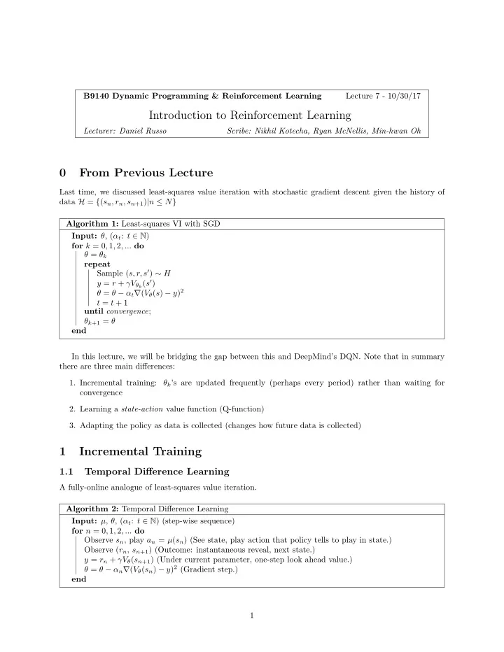
B9140 Dynamic Programming & Reinforcement Learning Lecture 7 - 10/30/17 Introduction to Reinforcement Learning Lecturer: Daniel Russo Scribe: Nikhil Kotecha, Ryan McNellis, Min-hwan Oh 0 From Previous Lecture Last time, we discussed least-squares value iteration with stochastic gradient descent given the history of data H = { ( s n , r n , s n +1 ) | n ≤ N } Algorithm 1: Least-squares VI with SGD Input: θ , ( α t : t ∈ N ) for k = 0 , 1 , 2 , ... do θ = θ k repeat Sample ( s, r, s ′ ) ∼ H y = r + γV θ k ( s ′ ) θ = θ − α t ∇ ( V θ ( s ) − y ) 2 t = t + 1 until convergence ; θ k +1 = θ end In this lecture, we will be bridging the gap between this and DeepMind’s DQN. Note that in summary there are three main differences: 1. Incremental training: θ k ’s are updated frequently (perhaps every period) rather than waiting for convergence 2. Learning a state-action value function (Q-function) 3. Adapting the policy as data is collected (changes how future data is collected) 1 Incremental Training 1.1 Temporal Difference Learning A fully-online analogue of least-squares value iteration. Algorithm 2: Temporal Difference Learning Input: µ , θ , ( α t : t ∈ N ) (step-wise sequence) for n = 0 , 1 , 2 , ... do Observe s n , play a n = µ ( s n ) (See state, play action that policy tells to play in state.) Observe ( r n , s n +1 ) (Outcome: instantaneous reveal, next state.) y = r n + γV θ ( s n +1 ) (Under current parameter, one-step look ahead value.) θ = θ − α n ∇ ( V θ ( s n ) − y ) 2 (Gradient step.) end 1

This mechanism is biologically plausible: instantaneous outcomes can be labeled good or bad with the goal of trying to predict if outcomes are good or bad. The realized y depends on the parameter, akin to trying to predict a moving target. Temporal Difference (TD) with linear function approximation converges to θ ∗ solving: Φ θ ∗ = Π T µ Φ θ ∗ (1) Result: (Tsitsiklis & Van Roy, 1997 1 ) -Fixed point of: V θ k +1 = Π T µ V θ k (2) This relies on the theory of stochastic approximation and fact that Π T µ is a contraction (recall proof from previous class). Essence of the result in 3 steps: Step 1, Calculate gradient: ( V θ ( S n ) − y ) 2 ∂ φ ( S n ) ⊤ θ − ( r n + γφ ( S n +1 ) ⊤ θ ) � � = φ ( S n ) = g n ( θ ) (3) ∂θ 2 In words, the gradient of the loss is equal to the predicted value less the reward and discounted predicted value with the feature value in the next state. This can also be expressed in the following equation, in which g n ( θ ) is a random variable that depends on the state and the realized reward and state. ( V θ ( S n ) − y ) 2 ∂ = g n ( θ ) (4) ∂θ 2 Step 2, Denoise: E 0 [( g n ( θ )] = Φ ⊤ D π ( T µ Φ θ − Φ θ ) (5) Here, the expectation is taken over the steady state. In the RHS, Φ represents the features, D π is a diagonal matrix with the steady state probabilites on the diagonal. Inside the parenthetical looks like the average Bellman error in prediction as measured in features. Step 3, Solution to fixed point equation: ( θ − θ ∗ ) ⊤ E 0 [ g n ( θ )] > 0 (6) Above is the essence of the result: looking at the convergence point, which is the solution to the fixed point equation. 1 Tsitsiklis, J. and Van Roy, B. (1997). An Analysis of Temporal-Difference Learning with Function Approximation. IEEE Transactions on Automatic Control, 42(5): 674- 690. 2

1.2 Stochastic Approximation History: Robbins and Monro, 1951 wrote a paper entitled “A Stochastic Approximation Method.” 2 These ideas are widely used in control systems, signal processing, stochastic simulation, time series, and Machine Learning (today). Incremental Mean: observe X 1 , X 2 , ...i.i.d with mean θ n � n − 1 � θ n = 1 X i = 1 θ n − 1 − 1 � � ˆ = ˆ ˆ = ˆ � � X i + X n θ n − 1 − X n θ n − 1 − α n ( g n ) (7) n n n i i Here time is represented by n . In the first step the empirical average is taken, then rewritten to exactly compute the mean. This results in the new mean being equal to the last mean less the difference of the mean estimate and the observation. Some key observations: Observation 1, the sum of squares is finite: ∞ ∞ � � α 2 α n = ∞ , n < ∞ (8) n =1 n =1 Observation 2, average updates go in the right direction: E [ g n |F n − 1 ] = (ˆ θ n − 1 − θ ) (9) To put these observations together, use the Martingale Convergence Theorem to show ˆ θ n → θ . As it turns out, the above procedure is equivalent to applying Stochastic Gradient Descent (SGD) to the objective function E [( θ − X ) 2 / 2] using step size α n = 1 /n . More generally, SGD is used to find the parameter θ which minimizes the nonnegative loss function ℓ ( θ ) = E ξ [ f ( θ, ξ )] for some f ( · , · ). It is assumed that this expectation cannot be computed directly. However, we can use SGD to optimize over the loss function with respect to i.i.d. samples of the random variable ξ . The SGD algorithm is as follows: Algorithm 3: Stochastic Gradient Descent (SGD) Input: step size α t , starting parameter θ 1 for t = 1 , 2 , ... do Sample ξ t ( i.i.d. ) Compute g t = ∇ θ f ( θ, ξ t ) | θ = θ t θ t +1 = θ t − α t g t end Let ∇ ℓ ( θ t ) be shorthand notation for ∇ ℓ ( θ ) | θ = θ t . If the step size α t is chosen appropriately, then SGD converges to a locally-optimal solution: Theorem 1. ||∇ ℓ ( θ t ) || → 0 as t → ∞ if the following conditions are satisfied: 1. � ∞ t =1 α t = ∞ 2. � ∞ t =1 α 2 t < ∞ 2 Robbins, H., & Monro, S. (1951). A stochastic approximation method. The annals of mathematical statistics, 400-407. 3

Proof (sketch): Let F t = { ξ s : s ≤ t } . Then, E [ g t |F t − 1 ] = ∇ ℓ ( θ t ): given the entire history of data F t − 1 , the expected value of the noisy gradient g t is equal to the true gradient ∇ ℓ ( θ ) | θ = θ t . One can also show that: ℓ ( θ t +1 ) = ℓ ( θ t ) − α t ∇ ℓ ( θ t ) ⊤ g t + O ( α 2 t ) Combining these two observations, E [ ℓ ( θ t ) − ℓ ( θ t +1 ) | F t − 1 ] = α t ||∇ ℓ ( θ t ) || 2 + O ( α 2 t ) Assume by contradiction that lim inf t →∞ ||∇ ℓ ( θ t ) || 2 = c > 0. Then, for large t , E [ ℓ ( θ t )] decreases by α t c + O ( α 2 t ) each iteration. This implies that E [ ℓ ( θ t )] approaches −∞ , given the theorem conditions t α 2 � t α t = ∞ and � t < ∞ . However, this violates the non-negativity of ℓ ( θ ). Thus, it must be the case that lim inf t →∞ ||∇ ℓ ( θ t ) || 2 = 0. 2 Using State-Action Value Functions Up to this point in class, we have focused on on the estimation of the value functions V ∗ ( s ) corresponding to the optimal policy. However, the reinforcement-learning literature instead focuses on estimating the “Q- functions” Q ∗ ( s, a ), which can be thought of as the “value” of a state-action pair. This shift in focus is due to the fact that reinforcement-learning algorithms need to do more than simply evaluate a fixed policy – they also need to control the data-collection process through the actions they take (this will be emphasized in the next section). However, as we will show, the methodology we have studied for estimating value functions extends easily to estimating Q-functions. First, note that the value function V ∗ ( s ) can be computed from the Q-function Q ∗ ( s, a ) in the following way: V ∗ ( s ) = max a ∈ A Q ∗ ( s, a ) (10) The Q-functions obey the following system of equations: Q ∗ ( s, a ) = R ( s, a ) + γ � P ( s, a, s ′ ) V ∗ ( s ′ ) (11) s ′ In words, Q ∗ ( s, a ) represents the reward from taking action a in state s plus the expected cost-to-go from taking actions according to the optimal policy. As it turns out, the optimal policy can be derived from knowing Q ∗ : µ ∗ ( s ) = arg max a ∈ A Q ∗ ( s, a ) Thus, if we can estimate Q ∗ , then we can simply read off the optimal policy. Note that we can define a Q -function with respect to any policy µ , rather than simply the optimal policy: � P ( s, a, s ′ ) V µ ( s ′ ) , Q µ ( s, a ) = R ( s, a ) + γ s ′ or, in words, the reward from taking action a in state s plus the expected cost-to-go from taking actions according to the policy µ . As mentioned previously, much of the theory about value functions extends to Q -functions. For example, Q ∗ obeys its own Bellman equations: Q ∗ ( s, a ) = R ( s, a ) + γ � P ( s, a, s ′ ) max a ∈ A Q ∗ ( s ′ , a ) s ′ 4