
SLIDE 1
Introduction to Machine Learning Linear Regression Models
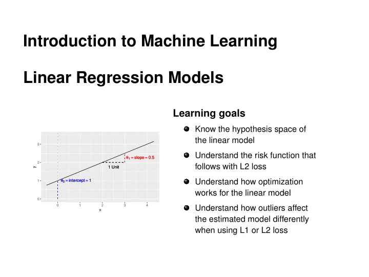
1 Unit 1 Unit θ1 = slope = 0.5 θ1 = slope = 0.5 θ0 = intercept = 1 θ0 = intercept = 1
1 2 3 1 2 3 4
x y
Introduction to Machine Learning Linear Regression Models Learning - - PowerPoint PPT Presentation
Introduction to Machine Learning Linear Regression Models Learning goals Know the hypothesis space of the linear model 3 Understand the risk function that 1 = slope = 0.5 1 = slope = 0.5 2 follows with L2 loss 1 Unit 1 Unit y 0 =
1 Unit 1 Unit θ1 = slope = 0.5 θ1 = slope = 0.5 θ0 = intercept = 1 θ0 = intercept = 1
1 2 3 1 2 3 4
x y
c
1 Unit 1 Unit θ1 = slope = 0.5 θ1 = slope = 0.5 θ0 = intercept = 1 θ0 = intercept = 1
1 2 3 1 2 3 4
x y
c
c
n
n
−1 1 1 2 3 4 5 6
x y
c
2 4 6 8 −2 2 4 6 θ = ( 1.8 , 0.3 ) SSE: 16.85 c
2 4 6 8 −2 2 4 6 θ = ( 1.8 , 0.3 ) SSE: 16.85 2 4 6 8 −2 2 4 6 θ = ( 1 , 0.1 ) SSE: 24.3 c
2 4 6 8 −2 2 4 6 θ = ( 1.8 , 0.3 ) SSE: 16.85 2 4 6 8 −2 2 4 6 θ = ( 1 , 0.1 ) SSE: 24.3 2 4 6 8 −2 2 4 6 θ = ( 0.5 , 0.8 ) SSE: 10.61 c
2 4 6 8 −2 2 4 6 θ = ( 1.8 , 0.3 ) SSE: 16.85 2 4 6 8 −2 2 4 6 θ = ( 1 , 0.1 ) SSE: 24.3 2 4 6 8 −2 2 4 6 θ = ( 0.5 , 0.8 ) SSE: 10.61 I n t e r c e p t −2 −1 1 2 Slope 0.0 0.5 1.0 1.5 S S E 20 40 60 80 100
c
Intercept −2 −1 1 2 S l
e 0.0 0.5 1.0 1.5 SSE 20 40 60 80 100 c
Intercept −2 −1 1 2 S l
e 0.0 0.5 1.0 1.5 SSE 20 40 60 80 100 c
2 4 6 8 −2 2 4 6 θ = ( 1.8 , 0.3 ) SSE: 16.85 2 4 6 8 −2 2 4 6 θ = ( 1 , 0.1 ) SSE: 24.3 2 4 6 8 −2 2 4 6 θ = ( 0.5 , 0.8 ) SSE: 10.61 2 4 6 8 −2 2 4 6 θ = ( −1.7 , 1.3 ) SSE: 5.88 I n t e r c e p t −2 −1 1 2 Slope 0.0 0.5 1.0 1.5 S S E 20 40 60 80 100
c
n
2
1 x(1)
1
p
1 x(2)
1
p
1 x(n)
1
p
c
n
n
Intercept −2 −1 1 2 S l
e 0.0 0.5 1.0 1.5 Sum of Absolute Errors 5 10 15 20
L1 Loss Surface
Intercept −2 −1 1 2 S l
e 0.0 0.5 1.0 1.5 SSE 20 40 60 80 100
L2 Loss Surface
c
25 50 75 100 2 4 6 8 10
x1 y Loss
L1 L2
L1 vs L2 Without Outlier
c
25 50 75 100 0.0 2.5 5.0 7.5 10.0
x1 y Loss
L1 L2
L1 vs L2 With Outlier
c
c