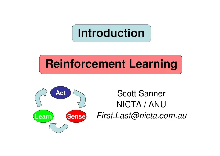
Introduction Reinforcement Learning Scott Sanner Act NICTA / ANU - - PowerPoint PPT Presentation

Introduction Reinforcement Learning

Scott Sanner NICTA / ANU First.Last@nicta.com.au

Sense Learn Act

Lecture Goals

1) To understand formal models for decision- making under uncertainty and their properties

• Unknown models (reinforcement learning)
• Known models (planning under uncertainty)

2) To understand efficient solution algorithms for these models

Applications

Elevator Control

• Concurrent Actions

– Elevator: up/down/stay – 6 elevators: 3^6 actions

• Dynamics:

– Random arrivals (e.g., Poisson)

• Objective:

– Minimize total wait – (Requires being proactive about future arrivals)

• Constraints:

– People might get annoyed if elevator reverses direction

Two-player Games

• Othello / Reversi

– Solved by Logistello! – Monte Carlo RL (self-play) + Logistic regression + Search

• Backgammon

– Solved by TD-Gammon! – Temporal Difference (self-play) + Artificial Neural Net + Search

• Go

– Learning + Search? – Unsolved!

Multi-player Games: Poker

• Multiagent (adversarial)
• Strict uncertainty

– Opponent may abruptly change strategy – Might prefer best outcome for any opponent strategy

• Multiple rounds (sequential)
• Partially observable!

– Earlier actions may reveal information – Or they may not (bluff)

DARPA Grand Challenge

• Autonomous mobile robotics

– Extremely complex task, requires expertise in vision, sensors, real-time operating systems

• Partially observable

– e.g., only get noisy sensor readings

• Model unknown

– e.g., steering response in different terrain

How to formalize these problems?

Observations, States, & Actions

Observations State Actions

Observations and States

• Observation set O

– Perceptions, e.g.,

• Distance from car to edge of road
• My opponent’s bet in Poker
• State set S

– At any point in time, system is in some state, e.g.,

• Actual distance to edge of road
• My opponent’s hand of cards in Poker

– State set description varies between problems

• Could be all observation histories
• Could be infinite (e.g., continuous state description)

Agent Actions

• Action set A

– Actions could be concurrent – If k actions, A = A1 × × × × … × × × × Ak

• Schedule all deliveries to be made at 10am

– All actions need not be under agent control

• Other agents, e.g.,

– Alternating turns: Poker, Othello – Concurrent turns: Highway Driving, Soccer

• Exogenous events due to Nature, e.g.,

– Random arrival of person waiting for elevator – Random failure of equipment

• {history} encodes all prev. observations, actions

Observation Function

• Z: {history} ×

× × × O → → → → [0,1]

• Not observable: (used in conformant planning)

– O = ∅ ∅ ∅ ∅ – e.g., heaven vs. hell » only get feedback once you meet St. Pete

• Fully observable:

– S ↔ O … the case we focus on! – e.g., many board games, » Othello, Backgammon, Go

• Partially observable:

– all remaining cases – also called incomplete information in game theory – e.g., driving a car, Poker

Transition Function

• T: {history}×

× × ×A× × × ×S→ → → →[0,1]

– Some properties

• Stationary: T does not change over time
• Markovian: T: S × A × S → [0,1]

– Next state dependent only upon previous state / action – If not Markovian, can always augment state description » e.g., elevator traffic model differs throughout day; so encode time in S to make T Markovian!

Goals and Rewards

• Goal-oriented rewards

– Assign any reward value s.t. R(success) > R(fail) – Can have negative costs C(a) for action a

• Known as stochastic shortest path problems
• What if multiple (or no) goals?

– How to specify preferences? – R(s,a) assigns utilities to each state s and action a

• Then maximize expected utility

… but how to trade off rewards over time?

Optimization: Best Action when s=1?

• Must define objective criterion to optimize!

– How to trade off immediate vs. future reward? – E.g., use discount factor γ (try γ=.9 vs. γ=.1)

• a=stay

a=stay

• a=stay

a=stay

• a=stay

a=stay

Trading Off Sequential Rewards

• Sequential-decision making objective

– Horizon

• Finite: Only care about h-steps into future
• Infinite: Literally; will act same today as tomorrow

– How to trade off reward over time?

• Expected average cumulative return
• Expected discounted cumulative return

– Use discount factor γ » Reward t time steps in future discounted by γt – Many interpretations » Future reward worth less than immediate reward

» (1-γ) chance of termination at each time step

• Important property:

» cumulative reward finite

Knowledge of Environment

• Model-known:

– Know Z, T, R – Called: Planning (under uncertainty)

• Planning generally assumed to be goal-oriented
• Decision-theoretic if maximizing expected utility
• Model-free:

– At least one of Z, T, R unknown – Called: Reinforcement learning

• Have to interact with environment to obtain samples of Z, T, R
• Use R samples as reward reinforcement to optimize actions
• Can still approximate model in model-free case

– Permits hybrid planning and learning

Saves expensive interaction!

Finally a Formal Model

• Environment model:
• S,O,A,Z,T,R
• – General characteristics
• Stationary and Markov transitions?
• Number of agents (1, 2, 3+)
• Observability (full, partial, none)

– Objective

• Horizon
• Average vs. discounted (γ)

– Model-based or model-free

• Different assumptions yield well-studied models

– Markovian assumption on T frequently made (MDP)

• Different properties of solutions for each model

– That’s what this lecture is about!

Can you provide this description for five previous examples? Note: Don’t worry about solution just yet, just formalize problem.

MDPs and Model-based Solutions Reinforcement Learning

Scott Sanner NICTA / ANU First.Last@nicta.com.au

Sense Learn Act

MDPs S,A,T,R,γ

• S = {1,2}; A = {stay, change}
• Reward

– R(s=1,a=stay) = 2 – …

• Transitions
• – …
• Discount γ
• (P=1.0)

(P=1.0)

• (P=1.0)

(P=1.0)

• (P=1.0)

(P=1.0)

• How to act

in an MDP? Define policy π: S → A Note: fully

• bservable

What’s the best Policy?

• Must define reward criterion to optimize!

– Discount factor γ important (γ=.9 vs. γ=.1)

• a=stay (P=.9)

a=stay (P=.9)

• a=stay (P=.9)

a=stay (P=.9)

• a=stay (P=.9)

a=stay (P=.9)

MDP Policy, Value, & Solution

• Define value of a policy π:
• Tells how much value you expect to get by

following π starting from state s

• Allows us to define optimal solution:

– Find optimal policy π* that maximizes value – Surprisingly: – Furthermore: always a deterministic π*

Value Function → Policy

• Given arbitrary value V (optimal or not)…

– A greedy policy πV takes action in each state that maximizes expected value w.r.t. V: – If can act so as to obtain V after doing action a in state s, πV guarantees V(s) in expectation

• If V not optimal, but a lower bound on V*,

πV guarantees at least that much value!

Value Iteration: from finite to ∞ decisions

• Given optimal t-1-stage-to-go value function
• How to act optimally with t decisions?

– Take action a then act so as to achieve Vt-1 thereafter – What is expected value of best action a at decision stage t? – At ∞ horizon, converges to V* – This value iteration solution know as dynamic programming (DP)

• Make sure you

can derive these equations from first principles!

Bellman Fixed Point

• Define Bellman backup operator B:
• ∃ an optimal value function V* and an optimal

deterministic greedy policy π*= πV* satisfying:

• Vt-1

Vt

Bellman Error and Properties

• Define Bellman error BE:
• Clearly:
• Can prove B is a contraction operator for BE:
• Hmmm…. Does

this suggest a solution?

Value Iteration: in search of fixed-point

• Start with arbitrary value function V0
• Iteratively apply Bellman backup
• Bellman error decreases on each iteration

– Terminate when – Guarantees ε-optimal value function

• i.e., Vt within ε of V* for all states

Precompute maximum number of steps for ε?

• Look familiar?

Same DP solution as before.

Single Dynamic Programming (DP) Step

• Graphical view:

s1 a1 a2 s1 s2 s3 s2

Synchronous DP Updates (Value Iteration)

MAX 2

S

1

S

2

S

1

S

2

S

2

A1 A2 A1 A2 A1 A2 A1 A2 A1 A2 A1 A2 S

1

V (s )

2

S

1 1 1 1

V (s )

1 1

V (s ) V (s ) V (s )

1

V (s ) V (s )

2 3 2 2 2 2

V (s )

3 MAX MAX MAX MAX MAX

S

Asynchronous DP Updates (Asynchronous Value Iteration)

...

1

A2 A1

1

V (s )

1

S

2

S

1

S

1

S

2

A2 A1

MAX

S

2

S

1 1

V (s )

1

V (s )

MAX 1

V (s )

3 2

... ...

S

Don’t need to update values synchronously with uniform depth. As long as each state updated with non-zero probability, convergence still guaranteed! Can you see intuition for error contraction?

Real-time DP (RTDP)

• Async. DP guaranteed to converge over relevant states

– relevant states: states reachable from initial states under π* – may converge without visiting all states!

Prioritized Sweeping (PS)

• Simple asynchronous DP idea

– Focus backups on high error states – Can use in conjunction with other focused methods, e.g., RTDP

• Every time state visited:

– Record Bellman error of state – Push state onto queue with priority = Bellman error

• In between simulations / experience, repeat:

– Withdraw maximal priority state from queue – Perform Bellman backup on state

• Record Bellman error of predecessor states
• Push predecessor states onto queue with priority = Bellman error

Where do RTDP and PS each focus?

Which approach is better?

• Synchronous DP Updates

– Good when you need a policy for every state – OR transitions are dense

• Asynchronous DP Updates

– Know best states to update

• e.g., reachable states, e.g. RTDP
• e.g., high error states, e.g. PS

– Know how to order updates

• e.g., from goal back to initial state if DAG

Policy Evaluation

• Given π, how to derive Vπ?
• Matrix inversion
• Set up linear equality (no max!) for each state
• Can solve linear system in vector form as follows
• Successive approximation
• Essentially value iteration with fixed policy
• Initialize Vπ

0 arbitrarily

• Guaranteed to converge to Vπ
• Guaranteed

invertible.

Policy Iteration

!" # $ # % &' ' ( ) # # # *

• ' ' '
• +

,

Modified Policy Iteration

• Value iteration

– Each iteration seen as doing 1-step of policy evaluation for current greedy policy – Bootstrap with value estimate of previous policy

• Policy iteration

– Each iteration is full evaluation of Vπ for current policy π – Then do greedy policy update

• Modified policy iteration

– Like policy iteration, but Vπi need only be closer to V* than Vπi-1

• Fixed number of steps of successive approximation for Vπi suffices

when bootstrapped with Vπi-1

– Typically faster than VI & PI in practice

Conclusion

• Basic introduction to MDPs

– Bellman equations from first principles – Solution via various algorithms

• Should be familiar with model-based solutions

– Value Iteration

• Synchronous DP
• Asynchronous DP (RTDP, PS)

– (Modified) Policy Iteration

• Policy evaluation
• Model-free solutions just sample from above

Model-free MDP Solutions Reinforcement Learning

Scott Sanner NICTA / ANU First.Last@nicta.com.au

Sense Learn Act

Chapter 5: Monte Carlo Methods

• Monte Carlo methods learn from sample returns

– Sample from

• experience in real application, or
• simulations of known model

– Only defined for episodic (terminating) tasks – On-line: Learn while acting

Slides from Rich Sutton’s course CMP499/609 Reinforcement Learning in AI

http://rlai.cs.ualberta.ca/RLAI/RLAIcourse/RLAIcourse2007.html

Reinforcement Learning, Sutton & Barto, 1998. Online.

Essence of Monte Carlo (MC)

• MC samples directly from value expectation for

each state given π

Monte Carlo Policy Evaluation

• Goal: learn Vπ(s)
• Given: some number of episodes under π which

contain s

• Idea: Average returns observed after visits to s

1 2 3 4 5

Start Goal update each state with final discounted return

Monte Carlo policy evaluation

Blackjack example

• Object: Have your card sum be greater than the

dealer’s without exceeding 21.

• States (200 of them):

– current sum (12-21) – dealer’s showing card (ace-10) – do I have a useable ace?

• Reward: +1 win, 0 draw, -1 lose
• Actions: stick (stop receiving cards),

hit (receive another card)

• Policy: Stick if my sum is 20 or 21, else hit

Assuming fixed policy for now.

Blackjack value functions

Backup diagram for Monte Carlo

• Entire episode included
• Only one choice at each

state (unlike DP)

• MC does not bootstrap
• Time required to estimate
• ne state does not

depend on the total number of states

terminal state

MC Control: Need for Q-values

• Control: want to learn a good policy

– Not just evaluate a given policy

• If no model available

– Cannot execute policy based on V(s) – Instead, want to learn Q*(s,a)

• Qπ(s,a) - average return starting from state s and

action a following π

Monte Carlo Control

• MC policy iteration: Policy evaluation using MC

methods followed by policy improvement

• Policy improvement step: Greedy π’(s) is action

a maximizing Qπ(s,a)

π Q

evaluation improvement Q → Qπ π→

greedy(Q)

Instance of Generalized Policy Iteration.

Convergence of MC Control

• Greedy policy update improves or keeps value:
• This assumes all Q(s,a) visited an infinite

number of times

– Requires exploration, not just exploitation

• In practice, update policy after finite iterations

Blackjack Example Continued

• MC Control with exploring starts…
• Start with random (s,a) then follow π

Monte Carlo Control

) ( 1 s A ε ε + −

greedy ) (s A ε non-max

• How do we get rid of exploring starts?

– Need soft policies: π(s,a) > 0 for all s and a – e.g. ε-soft policy:

• Similar to GPI: move policy towards

greedy policy (i.e. ε-soft)

• Converges to best ε-soft policy

Summary

• MC has several advantages over DP:

– Learn from direct interaction with environment – No need for full models – Less harm by Markovian violations

• MC methods provide an alternate policy

evaluation process

• No bootstrapping (as opposed to DP)

Temporal Difference Methods Reinforcement Learning

Scott Sanner NICTA / ANU First.Last@nicta.com.au

Sense Learn Act

Chapter 6: Temporal Difference (TD) Learning

• Rather than sample full returns as in

Monte Carlo… TD methods sample Bellman backup

Slides from Rich Sutton’s course CMP499/609 Reinforcement Learning in AI

http://rlai.cs.ualberta.ca/RLAI/RLAIcourse/RLAIcourse2007.html

Reinforcement Learning, Sutton & Barto, 1998. Online.

TD Prediction

Simple every - visit Monte Carlo method : V(st ) ← V(st) +α Rt − V(st )

[ ]

Policy Evaluation (the prediction problem): for a given policy π, compute the state-value function V

π

Recall:

The simplest TD method, TD(0) : V(st ) ← V(st) +α rt+1 + γ V(st+1) − V(st )

[ ]

target: the actual return after time t target: an estimate of the return

Simple Monte Carlo

T T T T T T T T T T

V(st ) ← V(st) +α Rt − V (st )

[ ]

where R

t is the actual return following state st.

st

T T T T T T T T T T

Simplest TD Method

T T T T T T T T T T

st+1 r

t+1

st

V(st ) ← V(st) +α rt +1 + γ V (st+1) − V(st )

[ ]

T T T T T T T T T T

• cf. Dynamic Programming

V(st ) ← Eπ r

t +1 +γ V(st )

{ }

T T T T

st

r

t+1

st+1

T T T T T T T T T

TD methods bootstrap and sample

• Bootstrapping: update with estimate

– MC does not bootstrap – DP bootstraps – TD bootstraps

• Sampling:

– MC samples – DP does not sample – TD samples

Example: Driving Home

Stat e Elapsed T ime (minu tes) Pr edicted Time to Go Pr edicted Tota l Tim e leaving o ffice 30 30 reach car, ra ining 5 35 40 exit highway 20 15 35 beh ind truck 30 10 40 home street 40 3 43 arrive ho me 43 43

(5) (15) (10) (10) (3)

Driving Home

road

30 35 40 45

Predicted total travel time

leaving

• ffice

exiting highway 2ndary home arrive

Situation

actual outcome

reach car street home

Changes recommended by Monte Carlo methods (α=1) Changes recommended by TD methods (α=1)

Advantages of TD Learning

• TD methods do not require a model of the

environment, only experience

• TD, but not MC, methods can be fully

incremental

– You can learn before knowing the final outcome

• Less memory
• Less peak computation

– You can learn without the final outcome

• From incomplete sequences
• Both MC and TD converge, but which is faster?

Random Walk Example

A B C D E

1

start

Values learned by TD(0) after various numbers of episodes

TD and MC on the Random Walk

Data averaged over 100 sequences of episodes

Optimality of TD(0)

Batch Updating: train completely on a finite amount of data,

e.g., train repeatedly on 10 episodes until convergence. Only update estimates after complete pass through the data. For any finite Markov prediction task, under batch updating, TD(0) converges for sufficiently small α. Constant-α MC also converges under these conditions, but to a different answer!

Random Walk under Batch Updating

.0 .05 .1 .15 .2 .25

25 50 75 100

TD MC BATCH TRAINING Walks / Episodes RMS error, averaged

• ver states

After each new episode, all previous episodes were treated as a batch, and algorithm was trained until convergence. All repeated 100 times.

You are the Predictor

Suppose you observe the following 8 episodes: A, 0, B, 0 B, 1 B, 1 B, 1 B, 1 B, 1 B, 1 B, 0

V(A)? V(B)?

You are the Predictor

A B

r = 1 100% 75% 25% r = 0 r = 0

V(A)?

You are the Predictor

• The prediction that best matches the training

data is V(A)=0

– This minimizes the mean-square-error – This is what a batch Monte Carlo method gets

• If we consider the sequential aspect of the

problem, then we would set V(A)=.75

– This is correct for the maximum likelihood estimate

• f a Markov model generating the data

– This is what TD(0) gets

MC and TD results are same in ∞ limit of data. But what if data < ∞?

Sarsa: On-Policy TD Control

Turn this into a control method by always updating the policy to be greedy with respect to the current estimate:

SARSA = TD(0) for Q functions.

Q-Learning: Off-Policy TD Control

One - step Q - learning: Q st, at

( )← Q st, at ( )+ α r

t +1 +γ max a Q st+1, a

( )− Q st, at ( )

[ ]

Cliffwalking

ε−greedy, ε = 0.1 Optimal exploring policy. Optimal policy, but exploration hurts more here.

Practical Modeling: Afterstates

• Usually, a state-value function evaluates states

in which the agent can take an action.

• But sometimes it is useful to evaluate states

after agent has acted, as in tic-tac-toe.

• Why is this useful?
• An afterstate is really

just an action that looks like a state

X O X X O

+

X O

+

X X

Summary

• TD prediction
• Introduced one-step tabular model-free TD

methods

• Extend prediction to control

– On-policy control: Sarsa (instance of GPI) – Off-policy control: Q-learning

• These methods sample from Bellman backup,

combining aspects of DP and MC methods

a.k.a. bootstrapping

TD(λ λ λ λ): Between TD and MC Reinforcement Learning

Scott Sanner NICTA / ANU First.Last@nicta.com.au

Sense Learn Act

Unified View

Is there a hybrid

• f TD & MC?

Chapter 7: TD(λ)

• MC and TD estimate same value

– More estimators between two extremes

• Idea: average multiple estimators

– Yields lower variance – Leads to faster learning

Slides from Rich Sutton’s course CMP499/609 Reinforcement Learning in AI

http://rlai.cs.ualberta.ca/RLAI/RLAIcourse/RLAIcourse2007.html

Reinforcement Learning, Sutton & Barto, 1998. Online.

N-step TD Prediction

• Idea: Look farther into the future when you

do TD backup (1, 2, 3, …, n steps)

All of these estimate same value!

• Monte Carlo:
• TD:

– Use V to estimate remaining return

• n-step TD:

– 2 step return: – n-step return:

N-step Prediction

• Rt = r

t +1 + γr t +2 + γ 2r t +3 ++ γ T −t−1r T

Rt

(1) = r t +1 + γVt(st +1)

Rt

(2) = r t +1 + γr t +2 + γ 2Vt(st +2)

• Rt

(n ) = r t+1 + γr t+2 + γ 2r t +3 ++ γ n−1r t+n + γ nVt(st+n)

Random Walk Examples

• How does 2-step TD work here?
• How about 3-step TD?

Hint: TD(0) is 1-step return… update previous state on each time step.

A Larger Example

• Task: 19 state

random walk

• Do you think

there is an

• ptimal n?

for everything?

Averaging N-step Returns

• n-step methods were introduced to

help with TD(λ) understanding

• Idea: backup an average of several

returns

– e.g. backup half of 2-step & 4-step

• Called a complex backup

– Draw each component – Label with the weights for that component

Rt

avg = 1

2 Rt

(2) + 1

2 Rt

(4)

One backup

Forward View of TD(λ)

• TD(λ) is a method for

averaging all n-step backups

– weight by λn-1 (time since visitation) λ-return:

• Backup using λ-return:

Rt

λ = (1− λ)

λn−1

n=1 ∞

• Rt

(n)

∆Vt(st) = α Rt

λ −Vt(st)

[ ]

What happens when λ=1, λ= 0?

λ-return Weighting Function

Rt

λ = (1− λ)

λn−1

n=1 T −t−1

• Rt

(n) + λ T −t−1Rt

Until termination After termination

Forward View of TD(λ)

• Look forward from each state to determine

update from future states and rewards:

λ-return on the Random Walk

• Same 19 state random walk as before
• Why do you think intermediate values of λ

are best?

Backward View

• Shout δt backwards over time
• The strength of your voice decreases

with temporal distance by γλ

δt = r

t +1 + γVt(st +1) −Vt(st)

Backward View of TD(λ)

• The forward view was for theory
• The backward view is for mechanism
• New variable called eligibility trace

– On each step, decay all traces by γλ and increment the trace for the current state by 1 – Accumulating trace

et(s) ∈ ℜ+

et(s) = γλet−1(s) if s ≠ st γλet−1(s) +1 if s = st

On-line Tabular TD(λ)

Initialize V(s) arbitrarily Repeat (for each episode): e(s) = 0, for all s ∈ S Initialize s Repeat (for each step of episode): a ← action given by π for s Take action a, observe reward, r, and next state ′ s δ ← r + γV( ′ s ) −V(s) e(s) ← e(s) +1 For all s: V(s) ← V(s) + αδe(s) e(s) ← γλe(s) s ← ′ s Until s is terminal

Forward View = Backward View

• The forward (theoretical) view of averaging returns in

TD(λ) is equivalent to the backward (mechanistic) view for off-line updating

• The book shows:

∆Vt

TD(s) t= 0 T −1

• =

α

t= 0 T −1

Isst

(γλ)k−tδk

k= t T −1

• ∆Vt

λ(st)Isst t= 0 T −1

• =

α

t= 0 T −1

Isst

(γλ)k−tδk

k= t T −1

• ∆Vt

TD(s) t= 0 T −1

• =

∆Vt

λ(st) t= 0 T −1

• Isst

Backward updates Forward updates

algebra shown in book

On-line versus Off-line on Random Walk

• Same 19 state random walk
• On-line better over broader range of params

– Updates used immediately

Save all updates for end of episode.

Control: Sarsa(λ)

• Save eligibility for

state-action pairs instead of just states

et(s,a) = γλet−1(s,a) +1 if s = st and a = at γλet−1(s,a)

• therwise
• Qt +1(s,a) = Qt(s,a) + αδtet(s,a)

δt = r

t+1 + γQt(st +1,at+1) − Qt(st,at)

Sarsa(λ) Algorithm

Initialize Q(s,a) arbitrarily Repeat (for each episode) : e(s,a) = 0, for all s,a Initialize s,a Repeat (for each step of episode) : Take action a, observe r, ′ s Choose ′ a from ′ s using policy derived from Q (e.g. ε - greedy) δ ← r + γQ( ′ s , ′ a ) − Q(s,a) e(s,a) ← e(s,a) + 1 For all s,a : Q(s,a) ← Q(s,a) + αδe(s,a) e(s,a) ← γλe(s,a) s ← ′ s ;a ← ′ a Until s is terminal

Sarsa(λ) Gridworld Example

• With one trial, the agent has much more

information about how to get to the goal

– not necessarily the best way

• Can considerably accelerate learning

Replacing Traces

• Using accumulating traces, frequently visited

states can have eligibilities greater than 1

– This can be a problem for convergence

• Replacing traces: Instead of adding 1 when you

visit a state, set that trace to 1

et(s) = γλet−1(s) if s ≠ st 1 if s = st

Why Replacing Traces?

• Replacing traces can significantly speed learning
• Perform well for a broader set of parameters
• Accumulating traces poor for certain types of tasks:

Why is this task particularly

• nerous for accumulating traces?

Replacing Traces Example

• Same 19 state random walk task as before
• Replacing traces perform better than

accumulating traces over more values of λ

The Two Views

Averaging estimators. Efficient implementation Advantage of backward view for continuing tasks?

Conclusions

• TD(λ) and eligibilities

– efficient, incremental way to interpolate between MC and TD

• Averages multiple noisy estimators

– Lower variance – Faster learning

• Can significantly speed learning
• Does have a cost in computation

Practical Issues and Discussion Reinforcement Learning

Scott Sanner NICTA / ANU First.Last@nicta.com.au

Sense Learn Act

Need for Exploration in RL

• For model-based (known) MDP solutions

– Get convergence with deterministic policies

• But for model-free RL…

– Need exploration – Usually use stochastic policies for this

• Choose exploration action with small probability

– Then get convergence to optimality

Why Explore?

• Why do we need exploration in RL?

– Convergence requires all state/action values updated

• Easy when model-based

– Update any state as needed

• Harder when model-free (RL)

– Must be in a state to take a sample from it

• Current best policy may not explore all states…

– Must occasionally divert from exploiting best policy – Exploration ensures all reachable states/actions updated with non-zero probability

Key property, cannot guarantee convergence to π* otherwise!

Two Types of Exploration (of many)

• ε-greedy

– Select random action ε of the time

• Can decrease ε over time for convergence
• But should we explore all actions with same probability?
• Gibbs / Boltzmann Softmax
• Still selects all actions with non-zero probability
• Draw actions from
• More uniform as “temperature” τ → ∞
• More greedy as τ → 0

DP Updates vs. Sample Returns

• How to do updates?

– Another major dimension of RL methods

• MC uses full sample return
• TD(0) uses sampled DP backup (bootstrapping)
• TD(λ

λ λ λ) interpolates between TD(0) and MC=TD(1)

• .

The Great MC vs. TD(λ) Debate

• As we will see…

– TD(λ) methods generally learn faster than MC…

• Because TD(λ) updates value throughout episode
• MC has to wait until termination of episode
• But MC methods are robust to MDP violations

– non-Markovian models:

• MC methods can also be used to evaluate semi-MDPs

– Partially observable:

• MC methods can also be used to evaluate POMDP controllers
• Technically includes value function approximation methods

Why partially observable? B/c FA aliases states to achieve generalization. Proven that TD(λ) may not converge

Policy Evaluation vs. Control

Q-learning if λ λ λ λ=0 MC Off-policy Control Off-policy SARSA (GPI) MC On-policy Control (GPI) On-policy TD(λ λ λ λ) MC

• If learning Vπ (policy evaluation)

– Just use plain MC or TD(λ); always on-policy!

• For control case, where learning Qπ

– Terminology for off- vs. on-policy…

On- or off-policy Sampling Method

Summary: Concepts you should know

• Policy evaluation vs. control
• Exploration

– Where needed for RL.. which of above cases? – Why needed for convergence? – ε-greedy vs. softmax

• Advantage of latter?
• MC vs. TD(λ) methods

– Differences in sampling approach? – (Dis)advantages of each?

• Control in RL

– Have to learn Q-values, why? – On-policy vs. off-policy exploration methods

This is main web of

• ideas. From here,

it’s largely just implementation tricks of the trade.

RL with Function Approximation Reinforcement Learning

Scott Sanner NICTA / ANU First.Last@nicta.com.au

Sense Learn Act

General Function Approximation

• Posit f(θ,s)

– Can be linear, e.g., – Or non-linear, e.g., – Cover details in a moment…

• All we need is gradient

– In order to train weights via gradient descent

Gradient Descent

• Let f be any function of the parameter space.

Its gradient at any point

• θ

t in this space is:

∇

θ f (

• θ

t) = ∂f (

• θ

t)

∂θ(1) ,∂f (

• θ

t)

∂θ(2) ,,∂f (

• θ

t)

∂θ(n)

• T

.

θ(1) θ(2)

• θ

t = θt(1),θt(2)

( )

T

• θ

t+1 =

• θ

t −α∇ θ f (

• θ

t)

Iteratively move down the gradient:

Gradient Descent for RL

• Update parameters to minimize error

– Use mean squared error where – vt can be MC return – vt can be TD(0) 1-step sample

• At every sample, update is
• Make sure you

can derive this!

Gradient Descent for TD(λ)

• Eligibility now over parameters, not states

– So eligibility vector has same dimension as – Eligibility is proportional to gradient – TD error as usual, e.g. TD(0):

• Update now becomes
• Can you

justify this?

Linear-value Approximation

• Most popular form of function approximation

– Just have to learn weights (<< # states)

• Gradient computation?

Linear-value Approximation

• Warning, as we’ll see later…

– May be too limited if don’t choose right features

• But can add in new features on the fly

– Initialize parameter to zero

• Does not change value function
• Parameter will be learned with new experience

– Can even use overlapping (or hierarchical) features

• Function approximation will learn to trade off weights

– Automatic bias-variance tradeoff!

• Always use a regularizer (even when not adding features)

– Means: add parameter penalty to error, e.g.,

• Especially important when redundant features… why?

Nice Properties of Linear FA Methods

• The gradient for MSE is simple:

– For MSE, the error surface is simple:

• Linear gradient descent TD(λ) converges:

– Step size decreases appropriately – On-line sampling (states sampled from the on-policy distribution) – Converges to parameter vector with property:

• ∇

θ Vt(s) =

• φ

s

• θ

∞

• MSE(
• θ

∞) ≤ 1− γ λ

1− γ MSE(

• θ

∗)

best parameter vector

(Tsitsiklis & Van Roy, 1997) Slides from Rich Sutton’s course CMP499/609: http://rlai.cs.ualberta.ca/RLAI/RLAIcourse/RLAIcourse2007.html

Not control!

TicTacToe and Function Approximation

• Tic-Tac-Toe

– Approximate value function with – Let each fi be “an O in 1”, “an X in 9” – Will never learn optimal value

• Need conjunctions of multiple positions
• Linear function can do disjunction at best

X O

TicTacToe and Function Approximation

• How to improve performance?
• Better features

– adapt or generate them as you go along – E.g., conjunctions of other features

• Use a more powerful function approximator

– E.g., non-linear such as neural network – Latent variables learned at hidden nodes are boolean function expressive » encodes new complex features of input space

X O

Some Common Feature Classes…

Coarse Coding

σi

ci

σi

ci+1 ci-1 ci

σi+1

ci+1

Σ

θt

expanded representation, many features

• riginal

representation approximation

Slides from Rich Sutton’s course CMP499/609: http://rlai.cs.ualberta.ca/RLAI/RLAIcourse/RLAIcourse2007.html

Shaping Generalization in Coarse Coding

Slides from Rich Sutton’s course CMP499/609: http://rlai.cs.ualberta.ca/RLAI/RLAIcourse/RLAIcourse2007.html

Learning and Coarse Coding

10 40 160 640 2560 10240

Narrow features

desired function

Medium features Broad features

#Examples

approx- imation feature width

Slides from Rich Sutton’s course CMP499/609: http://rlai.cs.ualberta.ca/RLAI/RLAIcourse/RLAIcourse2007.html

Tile Coding

tiling #1 tiling #2

Shape of tiles ⇒ Generalization #Tilings ⇒ Resolution of final approximation

2D state space

Slides from Rich Sutton’s course CMP499/609: http://rlai.cs.ualberta.ca/RLAI/RLAIcourse/RLAIcourse2007.html

• Binary feature for each tile
• Number of features present

at any one time is constant

• Binary features means

weighted sum easy to compute

• Easy to compute indices of

the features present

But if state continuous… use continuous FA, not discrete tiling!

Tile Coding Cont.

• ne

tile

a) Irregular b) Log stripes c) Diagonal stripes

Irregular tilings Hashing

CMAC “Cerebellar model arithmetic computer” Albus 1971

Slides from Rich Sutton’s course CMP499/609: http://rlai.cs.ualberta.ca/RLAI/RLAIcourse/RLAIcourse2007.html

Radial Basis Functions (RBFs)

ci

σi

ci+1 ci-1

φs(i) = exp − s − ci

2

2σ i

2

• e.g., Gaussians

Slides from Rich Sutton’s course CMP499/609: http://rlai.cs.ualberta.ca/RLAI/RLAIcourse/RLAIcourse2007.html

Nonlinear Value-approximation

• Can use an artificial neural network (ANN)…

– Not convex, but good methods for training

• Learns latent features at hidden nodes

– Good if you don’t know what features to specify

• Easy to implement

– Just need derivative of parameters – Can derive via backpropagation

• Fancy name for the chain rule

TD-Gammon = TD(λ) + Function

• Approx. with ANNs

ANNs in a Nutshell

• Neural Net:

non-linear weighted combination of shared sub-functions

• Backpropagation:

to minimize SSE, train weights using gradient descent and chain rule

x0=1 x1 xn y1 ym

. . . . . .

h0=1

. . .

h1 hk all edges have weight wj,i

Σ Σ Σ Σ Σ Σ Σ Σ Σ Σ Σ Σ Σ Σ Σ Σ

Where the Real Problem Lies

• Function approximation often a necessity, which to use?

– MC – TD(λ) – TD xyz with adaptive lambda, etc…

• Algorithm choice can help (speed up) convergence

– But if features are inadequate – Or function approximation method is too restricted

• May never come close to optimal value (e.g., TicTacToe)
• Concerns for RL w/ FA:

– Primary: Good features, approximation architecture – Secondary: then (but also important) is convergence rate Note: TD(λ) may diverge for control! MC robust for FA, PO, Semi-MDPs.

Recap: FA in RL

• FA a necessity for most real-world problems

– Too large to solve exactly

• Space (curse of dimensionality)
• Time

– Utilize power of generalization!

• Introduces additional issue

– Not just speed of convergence

• As for exact methods

– But also features and approximation architecture

• Again: for real-world applications, this is arguably most

important issue to be resolved!

Conclusion Reinforcement Learning

Scott Sanner NICTA / ANU First.Last@nicta.com.au

Sense Learn Act

Lecture Goals

1) To understand formal models for decision- making under uncertainty and their properties

• Unknown models (reinforcement learning)
• Known models (planning under uncertainty)

2) To understand efficient solution algorithms for these models

Summary

• Lecture contents

– Modeling sequential decision making – Model-based solutions

• Value iteration, Policy iteration

– Model-free solutions

• Exploration, Control
• Monte Carlo, TD(λ)
• Function Approximation
• This is just the tip of the iceberg

– But a large chunk of the tip