
SLIDE 1
INTERPRETATION AND ESTIMATION OF DEFAULT CORRELATIONS
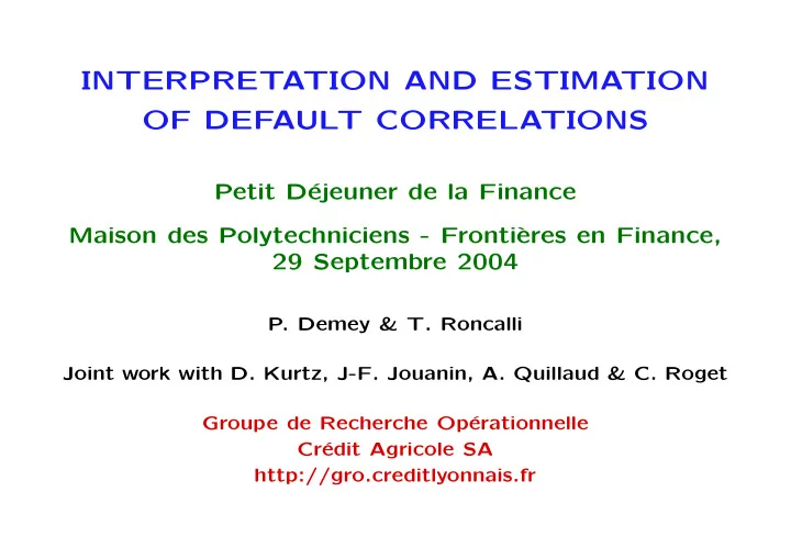
Petit D´ ejeuner de la Finance Maison des Polytechniciens - Fronti` eres en Finance, 29 Septembre 2004
- P. Demey & T. Roncalli
INTERPRETATION AND ESTIMATION OF DEFAULT CORRELATIONS Petit D - - PowerPoint PPT Presentation
INTERPRETATION AND ESTIMATION OF DEFAULT CORRELATIONS Petit D ejeuner de la Finance Maison des Polytechniciens - Fronti` eres en Finance, 29 Septembre 2004 P. Demey & T. Roncalli Joint work with D. Kurtz, J-F. Jouanin, A. Quillaud
Interpretation and Estimation of Default Correlations 1
Interpretation and Estimation of Default Correlations Motivations 1-1
Interpretation and Estimation of Default Correlations Motivations 1-2
Interpretation and Estimation of Default Correlations Default Correlations and Loss distribution of a Credit Book 2-1
Interpretation and Estimation of Default Correlations Default Correlations and Loss distribution of a Credit Book 2-2
Interpretation and Estimation of Default Correlations Default Correlations and Loss distribution of a Credit Book 2-3
Interpretation and Estimation of Default Correlations Default Correlations and Loss distribution of a Credit Book 2-4
Interpretation and Estimation of Default Correlations Default Correlations and Loss distribution of a Credit Book 2-5
Interpretation and Estimation of Default Correlations Default Correlations and Loss distribution of a Credit Book 2-6
Interpretation and Estimation of Default Correlations Default Correlations and Loss distribution of a Credit Book 2-7
Interpretation and Estimation of Default Correlations Default Correlations and Loss distribution of a Credit Book 2-8
t (1 − Pc (x))nc t−dc t
Interpretation and Estimation of Default Correlations Default Correlations and Loss distribution of a Credit Book 2-9
Default Correlations and Loss distribution of a Credit Book 2-10
Interpretation and Estimation of Default Correlations Default Correlations and Loss distribution of a Credit Book 2-11
t
t be the default rate at time t in class c.
Interpretation and Estimation of Default Correlations Default Correlations and Loss distribution of a Credit Book 2-12
Interpretation and Estimation of Default Correlations Default Correlations and Loss distribution of a Credit Book 2-13
Default Correlations and Loss distribution of a Credit Book 2-14
Interpretation and Estimation of Default Correlations Default Correlations and Loss distribution of a Credit Book 2-15
Interpretation and Estimation of Default Correlations Default Correlations and Credit Basket Pricing/Hedging 3-1
Interpretation and Estimation of Default Correlations Default Correlations and Credit Basket Pricing/Hedging 3-2
Interpretation and Estimation of Default Correlations Default Correlations and Credit Basket Pricing/Hedging 3-3
Start Wide Jump Recovery 28/10/2002 28/02/2003 Normal T4 AHOLD 40% 235 1205 970 CASINO 40% 235 152
SAINSBURY 40% 48 95 47 12
CARREFOUR 40% 60 47
KROGER 40% 127,5 108
SAFEWAY 40% 66,5 145 78,5 15
Correlation implied Start Wide Jump Recovery 20/02/2003 28/02/2003 Normal T4 AHOLD 40% 195 1205 1010 CASINO 40% 135 160 25
SAINSBURY 40% 68 95 27 3
CARREFOUR 40% 43 47 4 1
KROGER 40% 90 95 5 1
SAFEWAY 40% 195 145
Correlation implied
Interpretation and Estimation of Default Correlations Default Correlations and Credit Basket Pricing/Hedging 3-4
Start Wide Jump Recovery 05/07/2001 01/05/2002 Normal T4 WORLDCOM 15% 165 1700 1535 TELECOMI 15% 165 130
TELEFONI 15% 95 80
BELLSOUT 15% 47 75 28 9
BRITELEC 15% 105 105
MOTOROLA 15% 285 300 15 1
ATTCORP 15% 110 600 490 45 19 TELECOM 15% 185 345 160 15
Correlation implied
Start Wide Jump Recovery 13/08/2002 10/10/2002 Normal T4 TXU Corp. 40% 450 1250 800 SEMPRA 40% 275 400 125 7
DUKEENER 40% 170 225 55 5
VIVENENV 40% 170 152,5
SUEZ 40% 105 130 25 4
AMELECPO 40% 380 925 545 20
RWEAG 40% 67 98 31 6
ENEL 40% 68 87 19 4
Correlation implied
Interpretation and Estimation of Default Correlations Default Correlations and Credit Basket Pricing/Hedging 3-5
Interpretation and Estimation of Default Correlations Default Correlations and Credit Basket Pricing/Hedging 3-6
0,1 0,2 0,3 0,4 0,5 0,6 0,7 0,8 0,9 1 10 20 30 40 50 60 70 80 90 correlation pourcentage de pertes
tranche equity:0%->3% tranche mezanine:3%->12% tranche senior:12%->100%
tranche equity: 0%->3% tranche mezzanin: 3%->12% tranche senior:12%->100%
A B Upfront payment Running spread (bp) 0% 3% 34% 500 3% 6% 279 6% 9% 114 9% 12% 58 12% 22% 23
Interpretation and Estimation of Default Correlations Default Correlations and Credit Basket Pricing/Hedging 3-7
0,1 0,2 0,3 0,4 0,5 0,6 0,7 0,8 0%->3% 3%->6% 6%->9% 9%->12% 12%->22% tranches correlation implicite
corrélation implicite=0,04 corrélation implicite=0,75
Interpretation and Estimation of Default Correlations Default Correlations and Credit Basket Pricing/Hedging 3-8
0,05 0,1 0,15 0,2 0,25 0,3 0->3% 3->6% 6->9% 9->12% 12->22% 22->100% Tranches correlation implicite Betas corrélés Betas anticorrélés Betas=0,3
Interpretation and Estimation of Default Correlations Default Correlations and Credit Basket Pricing/Hedging 3-9