Insertion Sort Divide-And-Conquer Sorting Small instance. a[0] - - PDF document

Divide-And-Conquer Sorting

• Small instance.

n <= 1 elements. n <= 10 elements. We’ll use n <= 1 for now.

• Large instance.

Divide into k >= 2 smaller instances. k = 2, 3, 4, … ? What does each smaller instance look like? Sort smaller instances recursively. How do you combine the sorted smaller instances?

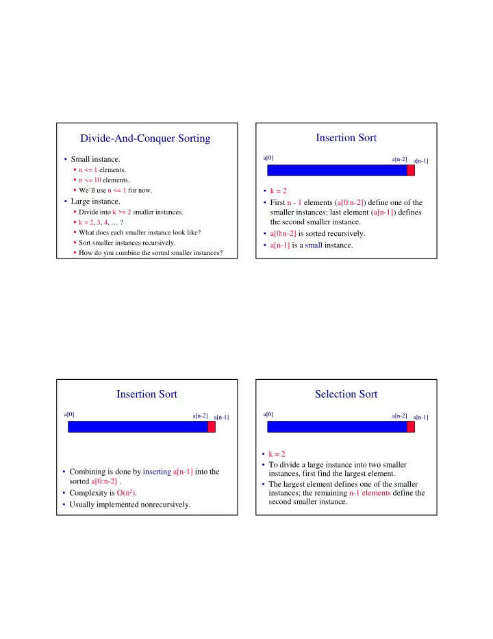
Insertion Sort

• k = 2
• First n - 1 elements (a[0:n-2]) define one of the

smaller instances; last element (a[n-1]) defines the second smaller instance.

• a[0:n-2] is sorted recursively.
• a[n-1] is a small instance.

a[0] a[0] a[n a[n-

• 1]

1] a[n a[n-

• 2]

2]

Insertion Sort

• Combining is done by inserting a[n-1] into the

sorted a[0:n-2] .

• Complexity is O(n2).
• Usually implemented nonrecursively.

a[0] a[0] a[n a[n-

• 1]

1] a[n a[n-

• 2]

2]

Selection Sort

• k = 2
• To divide a large instance into two smaller

instances, first find the largest element.

• The largest element defines one of the smaller

instances; the remaining n-1 elements define the second smaller instance.

a[0] a[0] a[n a[n-

• 1]

1] a[n a[n-

• 2]

2]

Selection Sort

• The second smaller instance is sorted recursively.
• Append the first smaller instance (largest

element) to the right end of the sorted smaller instance.

• Complexity is O(n2).
• Usually implemented nonrecursively.

a[0] a[0] a[n a[n-

• 1]

1] a[n a[n-

• 2]

2]

Bubble Sort

• Bubble sort may also be viewed as a k = 2 divide-

and-conquer sorting method.

• Insertion sort, selection sort and bubble sort

divide a large instance into one smaller instance

• f size n - 1 and another one of size 1.
• All three sort methods take O(n2) time.

Divide And Conquer

• Divide-and-conquer algorithms generally have

best complexity when a large instance is divided into smaller instances of approximately the same size.

• When k = 2 and n = 24, divide into two smaller

instances of size 12 each.

• When k = 2 and n = 25, divide into two smaller

instances of size 13 and 12, respectively.

Merge Sort

• k = 2
• First ceil(n/2) elements define one of the smaller

instances; remaining floor(n/2) elements define the second smaller instance.

• Each of the two smaller instances is sorted

recursively.

• The sorted smaller instances are combined using

a process called merge.

• Complexity is O(n log n).
• Usually implemented nonrecursively.

Merge Two Sorted Lists

• A = (2, 5, 6)

B = (1, 3, 8, 9, 10) C = ()

• Compare smallest elements of A and B and

merge smaller into C.

• A = (2, 5, 6)

B = (3, 8, 9, 10) C = (1)

Merge Two Sorted Lists

• A = (5, 6)

B = (3, 8, 9, 10) C = (1, 2)

• A = (5, 6)

B = (8, 9, 10) C = (1, 2, 3)

• A = (6)

B = (8, 9, 10) C = (1, 2, 3, 5)

Merge Two Sorted Lists

• A = ()

B = (8, 9, 10) C = (1, 2, 3, 5, 6)

• When one of A and B becomes empty, append

the other list to C.

• O(1) time needed to move an element into C.
• Total time is O(n + m), where n and m are,

respectively, the number of elements initially in A and B.

Merge Sort

[8, 3, 13, 6, 2, 14, 5, 9, 10, 1, 7, 12, 4] [8, 3, 13, 6, 2, 14, 5] [9, 10, 1, 7, 12, 4] [8, 3, 13, 6] [2, 14, 5] [8, 3] [13, 6] [8] [3][13] [6] [2, 14] [5] [2] [14] [9, 10, 1] [7, 12, 4] [9, 10] [1] [9] [10] [7, 12] [4] [7] [12]

Merge Sort

[3, 8] [6, 13] [3, 6, 8, 13] [8] [3][13] [6] [2, 14] [2, 5, 14] [2, 3, 5, 6, 8, 13, 14] [5] [2] [14] [9, 10] [1, 9, 10] [1] [9] [10] [7, 12] [4, 7, 12] [1, 4, 7, 9, 10,12] [1, 2, 3, 4, 5, 6, 7, 8, 9, 10, 12, 13,14] [4] [7] [12]

Time Complexity

• Let t(n) be the time required to sort n elements.
• t(0) = t(1) = c, where c is a constant.
• When n > 1,

t(n) = t(ceil(n/2)) + t(floor(n/2)) + dn, where d is a constant.

• To solve the recurrence, assume n is a power of 2

and use repeated substitution.

• t(n) = O(n log n).

Merge Sort

• Downward pass over the recursion tree.

Divide large instances into small ones.

• Upward pass over the recursion tree.

Merge pairs of sorted lists.

• Number of leaf nodes is n.
• Number of nonleaf nodes is n-1.

Time Complexity

• Downward pass.

O(1) time at each node. O(n) total time at all nodes.

• Upward pass.

O(n) time merging at each level that has a nonleaf node. Number of levels is O(log n). Total time is O(n log n).

Nonrecursive Version

• Eliminate downward pass.
• Start with sorted lists of size 1 and do

pairwise merging of these sorted lists as in the upward pass.

Nonrecursive Merge Sort

[8] [3] [13] [6] [2][14] [5] [9] [10] [1] [7] [12] [4] [3, 8] [6, 13] [2, 14] [5, 9] [1, 10] [7, 12] [4] [3, 6, 8, 13] [2, 5, 9, 14] [1, 7, 10, 12] [4] [2, 3, 5, 6, 8, 9, 13, 14] [1, 4, 7, 10, 12] [1, 2, 3, 4, 5, 6, 7, 8, 9, 10, 12, 13, 14]

Complexity

• Sorted segment size is 1, 2, 4, 8, …
• Number of merge passes is ceil(log2n).
• Each merge pass takes O(n) time.
• Total time is O(n log n).
• Need O(n) additional space for the merge.
• Merge sort is slower than insertion sort when n

<= 15 (approximately). So define a small instance to be an instance with n <= 15.

• Sort small instances using insertion sort.
• Start with segment size = 15.

Natural Merge Sort

• Initial sorted segments are the naturally ocurring

sorted segments in the input.

• Input = [8, 9, 10, 2, 5, 7, 9, 11, 13, 15, 6, 12, 14].
• Initial segments are:

[8, 9, 10] [2, 5, 7, 9, 11, 13, 15] [6, 12, 14]

• 2 (instead of 4) merge passes suffice.
• Segment boundaries have a[i] > a[i+1].

Quick Sort

• Small instance has n <= 1. Every small instance is a

sorted instance.

• To sort a large instance, select a pivot element from out
• f the n elements.
• Partition the n elements into 3 groups left, middle and

right.

• The middle group contains only the pivot element.
• All elements in the left group are <= pivot.
• All elements in the right group are >= pivot.
• Sort left and right groups recursively.
• Answer is sorted left group, followed by middle group

followed by sorted right group.

Example

6 2 8 5 11 10 4 1 9 7 3

Use 6 as the pivot.

2 8 5 11 10 4 1 9 7 3 6

Sort left and right groups recursively.

Choice Of Pivot

• Pivot is leftmost element in list that is to be sorted.

When sorting a[6:20], use a[6] as the pivot. Text implementation does this.

• Randomly select one of the elements to be sorted

as the pivot.

When sorting a[6:20], generate a random number r in the range [6, 20]. Use a[r] as the pivot.

Choice Of Pivot

• Median-of-Three rule. From the leftmost, middle,

and rightmost elements of the list to be sorted, select the one with median key as the pivot.

When sorting a[6:20], examine a[6], a[13] ((6+20)/2), and a[20]. Select the element with median (i.e., middle) key. If a[6].key = 30, a[13].key = 2, and a[20].key = 10, a[20] becomes the pivot. If a[6].key = 3, a[13].key = 2, and a[20].key = 10, a[6] becomes the pivot.

Choice Of Pivot

If a[6].key = 30, a[13].key = 25, and a[20].key = 10, a[13] becomes the pivot.

• When the pivot is picked at random or when the

median-of-three rule is used, we can use the quick sort code of the text provided we first swap the leftmost element and the chosen pivot.

pivot swap

Partitioning Into Three Groups

• Sort a = [6, 2, 8, 5, 11, 10, 4, 1, 9, 7, 3].
• Leftmost element (6) is the pivot.
• When another array b is available:

Scan a from left to right (omit the pivot in this scan), placing elements <= pivot at the left end of b and the remaining elements at the right end of b. The pivot is placed at the remaining position of the b.

Partitioning Example Using Additional Array

6 2 8 5 11 10 4 1 9 7 3

a b

2 8 5 11 10 4 1 9 7 3 6

Sort left and right groups recursively.

In-place Partitioning

• Find leftmost element (bigElement) > pivot.
• Find rightmost element (smallElement) <

pivot.

• Swap bigElement and smallElement

provided bigElement is to the left of smallElement.

• Repeat.

In-Place Partitioning Example

6 2 8 5 11 10 4 1 9 7 3

a

6 8 3 6 2 3 5 11 10 4 1 9 7 8

a

6 11 1 6 2 3 5 1 10 4 11 9 7 8

a

6 10 4 6 2 3 5 1 4 10 11 9 7 8

a

6 10 4

bigElement is not to left of smallElement, terminate process. Swap pivot and smallElement.

4 2 3 5 1 4 11 9 7 8

a

6 10 6

Complexity

• O(n) time to partition an array of n elements.
• Let t(n) be the time needed to sort n elements.
• t(0) = t(1) = c, where c is a constant.
• When t > 1,

t(n) = t(|left|) + t(|right|) + dn, where d is a constant.

• t(n) is maximum when either |left| = 0 or |right| =

0 following each partitioning.

Complexity

• This happens, for example, when the pivot is

always the smallest element.

• For the worst-case time,

t(n) = t(n-1) + dn, n > 1

• Use repeated substitution to get t(n) = O(n2).
• The best case arises when |left| and |right| are

equal (or differ by 1) following each partitioning.

• For the best case, the recurrence is the same as

for merge sort.

Complexity Of Quick Sort

• So the best-case complexity is O(n log n).
• Average complexity is also O(n log n).
• To help get partitions with almost equal size,

change in-place swap rule to:

Find leftmost element (bigElement) >= pivot. Find rightmost element (smallElement) <= pivot. Swap bigElement and smallElement provided bigElement is to the left of smallElement.

• O(n) space is needed for the recursion stack. May

be reduced to O(log n) (see Exercise 19.22).

Complexity Of Quick Sort

• To improve performance, define a small instance

to be one with n <= 15 (say) and sort small instances using insertion sort.

java.util.arrays.sort

• Arrays of a primitive data type are sorted using

quick sort.

n < 7 => insertion sort 7 <= n <= 40 => median of three n > 40 => pseudo median of 9 equally spaced elements

• divide the 9 elements into 3 groups
• find the median of each group
• pivot is median of the 3 group medians

java.util.arrays.sort

• Arrays of a nonprimitive data type are sorted using

merge sort.

n < 7 => insertion sort skip merge when last element of left segment is <= first element of right segment

• Merge sort is stable (relative order of elements

with equal keys is not changed).

• Quick sort is not stable.