Informed Search Chap. 4 Material in part from - - PDF document

1

Informed Search

Material in part from http://www.cs.cmu.edu/~awm/tutorials

• Chap. 4

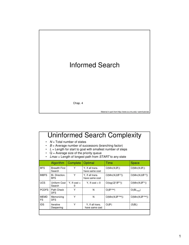
Uninformed Search Complexity

• N = Total number of states
• B = Average number of successors (branching factor)
• L = Length for start to goal with smallest number of steps
• Q = Average size of the priority queue
• Lmax = Length of longest path from START to any state

O(Min(N,2BL/2)) O(Min(N,2BL/2)) Y, If all trans. have same cost Y Bi- Direction. BFS BIBFS O(BL) O(BL) Y, If all trans. have same cost Y Iterative Deepening IDS O(Min(N,BLmax)) O(Min(N,BLmax)) N Y Memorizing DFS MEMD FS O(BLmax) O(BLmax) N Y Path Check DFS PCDFS O(Min(N,BC/ε)) O(log(Q)*BC/ε)) Y, If cost > 0 Y, If cost > Uniform Cost Search UCS O(Min(N,BL)) O(Min(N,BL)) Y, If all trans. have same cost Y Breadth First Search BFS

Space Time Optimal Complete Algorithm

2 states expanded so far

D E F

Search Revisited

1.Store a value f(s) at each state s 2.Choose the state with lowest f to expand next 3.Insert its successors If f(.) is chosen carefully, we will eventually find the lowest-cost sequence

START f(A) f(B) f(C) A B C

States ready to be expanded (the “fringe”)

START A B C f(A) f(B) f(C) D E F

Example:

• UCS (Uniform Cost Search): f(A) = g(A) = total cost of current

shortest path from START to A

• Store states awaiting expansion in a priority queue for efficient

retrieval of minimum f

• Optimal Guaranteed to find lowest cost sequence, but……

g(A) =10 g(A) =5

3

• Problem: No guidance as to how “far” any given state is from

the goal

• Solution: Design a function h(.) that gives us an estimate of the

distance between a state and the goal

START A B C GOAL h(A) = 3 h(B) = 6

Our best guess is that A is closer to GOAL than B so maybe it is a more promising state to expand

h(B) = 10

Heuristic Functions

• h(.) is a heuristic function for the search

problem

• h(s) = estimate of the cost of the shortest path

from s to GOAL

• h(.) cannot be computed solely from the states

and transitions in the current problem If we could, we would already know the optimal path!

• h(.) is based on external knowledge about the

problem informed search

• Questions:
• 1. Typical examples of h?
• 2. How to use h?
• 3. What are desirable/necessary properties of h?

4

Heuristic Functions Example

• h(s) = Euclidean distance to GOAL

X X x X

START GOAL The straight-line distance is lower from s than from s’ so maybe s has a better chance to be

• n the best path

s’ s

Heuristic Functions Example

• How could we define h(s)?

2 8 3 1 6 4 7 5 2 8 3 1 6 4 7 5

s

GOAL

5

First Attempt: Greedy Best First Search

• Simplest use of heuristic function: Always select the

node with smallest h(.) for expansion (i.e., f(s) = h(s)) Initialize PQ Insert START with value h(START) in PQ While (PQ not empty and no goal state is in PQ)

Pop the state s with the minimum value of h from PQ For all s’ in succs(s) If s’ is not already in PQ and has not already been visited Insert s’ in PQ with value h(s’)

Problem

• What solution do we find in this case?
• Greedy search clearly not optimal, even

though the heuristic function is non-stupid

START A B C GOAL h = 4 h = 3 h = 2 h = 1 h = 0 2 1 1 2 4

6

Trying to Fix the Problem

• g(s) is the cost from START to s only
• h(s) estimates the cost from s to GOAL
• Key insight: g(s) + h(s) estimates the total cost
• f the cheapest path from START to GOAL

going through s

• A* algorithm

START A B C GOAL h(A) = 3 f(A) = g(A) + h(A) = 13 g(A) = 10 h(B) = 6 f(B) = g(B) + h(B) = 11 g(A) = 5

Can A* Fix the Problem?

{(START,4)} {(A,5)} (f(A) = h(A) + g(A) = 3 + g(START) + cost(START, A) = 3 + 0 + 2) {(B,5) (C,7)} (f(C) = h(C) + g(C) = 1 + g(A) + cost(A, C) = 1 + 2 + 4) {(C,5)} (f(C) = h(C) + g(C) = 1 + g(B) + cost(B, C) = 1 + 3 + 1) {(GOAL,6)} START A B C GOAL h = 4 h = 3 h = 2 h = 1 h = 0 2 1 1 2 4

7

Can A* Fix the Problem?

{(START,4)} {(A,5)} (f(A) = h(A) + g(A) = 3 + g(START) + cost(START, A) = 3 + 0 + 2) {(B,5) (C,7)} (f(C) = h(C) + g(C) = 1 + g(A) + cost(A, C) = 1 + 2 + 4) {(C,5)} (f(C) = h(C) + g(C) = 1 + g(B) + cost(B, C) = 1 + 3 + 1) {(GOAL,6)} START A B C GOAL h = 4 h = 3 h = 2 h = 1 h = 0 2 1 1 2 4

C is placed in the queue with backpointers {A,START} A lower value of f(C) is found with backpointers {B,A,START}

• Termination condition
• Revisiting states
• Algorithm
• Optimality
• Avoiding revisiting states
• Choosing good heuristics
• Reducing memory usage

8

A* Termination Condition

• Stop when GOAL is popped from the queue!

Queue: {(B,4) (A,8)} {(C,4) (A,8)} {(D,4) (A,8)} {(A,8) (G,10)}

S A D B C G 1 1 1 1 7 1 h = 3 h = 2 h = 1 h = 7 h = 8

A* Termination Condition

• Stop when GOAL is popped from the queue!

Queue: {(B,4) (A,8)} {(C,4) (A,8)} {(D,4) (A,8)} {(A,8) (G,10)}

We have encountered G before we have a chance to visit the branch going through A. The problem is that at each step we use

• nly an estimate of

the path cost to the goal

S A D B C G 1 1 1 1 7 1 h = 3 h = 2 h = 1 h = 7 h = 8

9

Revisiting States

1 h = 7 A C B

START

D GOAL 1 1 1 7 h = 8 h = 3 h = 8 h = 1 1/2

A state that was already in the queue is re-visited. How is its priority updated?

Revisiting States

1 h = 7 A C B

START

D GOAL 1 1 1 7 h = 8 h = 3 h = 2 h = 1 1/2

A state that had been already expanded is re-visited. (Careful: This is a different example.)

10

A* Algorithm (inside loop)

Pop state s with lowest f(s) in queue If s = GOAL return SUCCESS Else expand s: For all s’ in succs (s): f’ = g(s’) + h(s’) = g(s) + cost(s,s’) + h(s’) If (s’ not seen before OR s’ previously expanded with f(s’) > f’ OR s’ in PQ with with f(s’) > f’) Promote/Insert s’ with new value f’ in PQ previous(s’)  s Else Ignore s’ (because it has been visited and its current path cost f(s’) is still the lowest path cost from START to s’)

Under what Conditions is A* Optimal?

• Problem: h(.) is a poor estimate of path

cost to the goal state

START

A

GOAL

h = 6 h = 7 1 1 3 {(START,6)} {(GOAL,3) (A,8)} Final path: {START, GOAL} with cost = 3

11

Admissible Heuristics

• Define h*(s) = the true minimal cost to the

goal from s

• h is admissible if

h(s) <= h*(s) for all states s

• In words: An admissible heuristic never
• verestimates the cost to the goal.

“Optimistic” estimate of cost to goal. A* is guaranteed to find the optimal path if h is admissible

Consistent (Monotonic) Heuristics h(s) <= h(s’) + cost(s,s’)

GOAL

s s’ Cost(s,s’) h(s’) h(s)

12

Consistent (Monotonic) Heuristics h(s) <= h(s’) + cost(s,s’)

GOAL

s s’ Cost(s,s’) h(s’) h(s)

Sort of triangular inequality implies that path cost always increases + need to expand node only once

Pop state s with lowest f(s) in queue If s = GOAL return SUCCESS Else expand s: For all s’ in succs (s): f’ = g(s’) + h(s’) = g(s) + cost(s,s’) + h(s’) If (s’ not seen before OR s’ previously expanded with f(s’) > f’ OR s’ in PQ with with f(s’) > f’) Promote/Insert s’ with new value f’ in PQ previous(s’)  s Else Ignore s’ (because it has been visited and its current path cost f(s’) is still the lowest path cost from START to s’)

I f h i s c

• n

s i s t e n t

13

Examples

GOAL

s h(s) For the navigation problem: The length of the shortest path is at least the distance between s and GOAL Euclidean distance is an admissible heuristic

2 8 3 1 6 4 7 5 2 8 3 1 6 4 7 5

s

GOAL

h(s) ? What about the puzzle?

Comparing Heuristics

• Overestimates A* performance because of the

tendency of IDS to expand states repeatedly

• Number of states expanded does not include

log() time access to queue

73 25 12 A* with heuristic h2 227 39 13 A* with heuristic h1 3.6 x 106 6,300 112 Iterative Deepening L = 12 steps L = 8 steps L = 4 steps

h1 = misplaced tiles h2 = Manhattan distance

Example from Russell&Norvig

14

5 4 3 6 1 8 7 2

s

2 8 3 1 6 4 7 5

GOAL h1(s) = 7 h2(s) = 2 + 3 + 3 + 2 + 4 + 2 + 0 + 2 = 18

Comparing Heuristics

h1(s) = 7 h2(s) = 2 + 3 + 3 + 2 + 4 + 2 + 0 + 2 = 18 h2 is larger than h1 and, at same time, A* seems to be more efficient with h2. Is there a connection between these two observations?

5 4 3 6 1 8 7 2

s

2 8 3 1 6 4 7 5

GOAL

h2 dominates h1 if h2(s) >= h1(s) for all s For any two heuristics h2 and h1 : If h2 dominates h1 then A* is more efficient (expands fewer states) with h2

Intuition: since h <= h*, a larger h is a better approximation of the true path cost

15

Limitations

• Computation: In the worst case, we may

have to explore all the states O(N)

• The good news: A* is optimally efficient

For a given h(.), no other optimal algorithm will expand fewer nodes

• The bad news: Storage is also potentially

large O(N)

IDS (Iterative Deepening Search)

• Need to make DFS optimal
• IDS (Iterative Deepening Search):

– Run DFS by searching only path of length 1 (DFS stops if length of path is greater than 1) – If that doesn’t find a solution, try again by running DFS on paths of length 2 or less – If that doesn’t find a solution, try again by running DFS on paths of length 3 or less – ……….. – Continue until a solution is found

16

Example: IDA* (Iterative Deepening A*)

• Same idea as Iterative Deepening DFS except use f(s) to

control depth of search instead of the number of transitions

• Example, assuming integer costs:
• 1. Run DFS, stopping at states s such that f(s) > 0

Stop if goal reached

• 2. Run DFS, stopping at states s such that f(s) > 1

Stop if goal reached

• 3. Run DFS, stopping at states s such that f(s) > 2

Stop if goal reached ……..Keep going by increasing the limit on f by 1 every time

• Complete (assuming we use loop-avoiding DFS)
• Optimal
• More expensive in computation cost than A*
• Memory order L as in DFS

Summary

• Informed search and heuristics
• First attempt: Best-First Greedy search
• A* algorithm

– Optimality – Condition on heuristic functions – Completeness – Limitations, space complexity issues – Extensions

Nils Nilsson. Problem Solving Methods in Artificial

• Intelligence. McGraw Hill (1971)

Judea Pearl. Heuristics: Intelligent Search Strategies for Computer Problem Solving (1984) Chapters 3&4 Russel & Norvig