information systems m prof paolo ciaccia http db deis
play

Information Systems M Prof. Paolo Ciaccia - PDF document

Information Systems M Prof. Paolo Ciaccia http://www-db.deis.unibo.it/courses/SI-M/ Time series, that is, sequences


  1. ��������������� Information Systems M Prof. Paolo Ciaccia http://www-db.deis.unibo.it/courses/SI-M/ ��������������������������� 
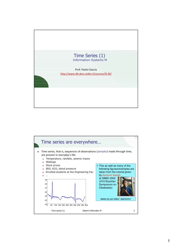
Time series, that is, sequences of observations ( samples ) made through time, � are present in everyday’s life: Temperature, rainfalls, seismic traces � Weblogs � Stock prices � This as well as many of the � EEG, ECG, blood pressure following figures/examples are � Enrolled students at the Engineering Fac. taken from the tutorial given � … by Eamonn Keogh � at SBBD 2002 29 (XVII Brazilian 28 Symposium on Databases) 27 26 25 www.cs.ucr.edu/~eamonn/ 24 23 0 50 100 150 200 250 300 350 400 450 500 ��������������� ��������������������� � 1

  2. �������������������������������������� Similarity search can help you in: � Looking for the occurrence of known patterns � Discovering unknown patterns � Putting “things together” (clustering) � Classifiying new data � Predicting/extrapolating future behaviors � … � ��������������� ��������������������� � ������������������������������� ��� Consider a large time series DB, e.g.: � 1 hour of ECG data: 1 GByte � Typical Weblog: 5 GBytes per week � Space Shuttle DB: 158 GBytes � MACHO Astronomical DB: 2 Tbytes, updated with 3 GBytes a day � (20 million stars recorded nightly for 4 years) http://wwwmacho.anu.edu.au/ First problem: large database size � Second problem: subjectivity of similarity evaluation � ��������������� ��������������������� ! 2

  3. "���������� ������������� Given two time series of equal length D, the usual way to measure their � (dis-)similarity is based on Euclidean distance However, with Euclidean distance we have to face two basic problems � 1. High9dimensionality: (very) large D values 2. Sensitivity to “alignment of values” s q For problem 1. we need to define � effective lower-bounding techniques that work in a (much) lower dimensional space ( ) D - 1 ( ) = ∑ − 2 L s, q s q For problem 2. we will introduce � 2 t t = t 0 a new similarity criterion ��������������� ��������������������� # $��%���������& Diretly comparing two time series (e.g., using Euclidean distance) might lead � to counter-intuitive results This is because Euclidean distance, as well as other measures, are very � sensitive to some data features that might conflict with the subjective notion of similarity Thus, a good idea is to pre-process time series in order to remove such � features ��������������� ��������������������� ' 3

  4. (����������������� Subtract from each sample the mean value of the series � 3 3 d(q,s) 2.5 2.5 2 2 1.5 1.5 1 1 0.5 0.5 0 0 0 50 100 150 200 250 300 0 50 100 150 200 250 300 q = q - mean(q) s = s - mean(s) d(q,s) 0 50 100 150 200 250 300 0 50 100 150 200 250 300 ��������������� ��������������������� ) *����� ���������& Normalize the amplitude (divide by the standard deviation of the series) � 0 100 200 300 400 500 600 700 800 900 1000 0 100 200 300 400 500 600 700 800 900 1000 q = (q - mean(q)) / std(q) s = (s - mean(s)) / std(s) ��������������� ��������������������� + 4

  5. ,������������ Average the values of each sample with those of its neighbors (smoothing) � 8 8 6 6 4 4 2 2 0 0 -2 -2 -4 -4 0 20 40 60 80 100 120 140 0 20 40 60 80 100 120 140 q = smooth(q) s = smooth(s) ��������������� ��������������������� - .����������������� �����/�.0����� The first method for reducing the dimensionality of time series, proposed in � [AFS93], was based on the Discrete Fourier Transform (DFT) Remind: given a time series s, the Fourier coefficients are complex numbers � (amplitude,phase), defined as: − 1 D 1 ∑ ( ) = − π = − S s exp j 2 f t/D f 0,..., D 1 f t D = t 0 Img Parseval theorem: DFT preserves the energy of the signal: � S f − ( ) ∑ − D 1 D 1 ( ) ∑ 2 = 2 = = E s s E S S |S f | t f t = 0 f = 0 Re where |S f | = |Re(S f ) + j Img(S f )| = √ (Re(S f ) 2 + Img(S f ) 2 ) is the absolute value of S f (its amplitude), which equals the Euclidean distance of S f from the origin ��������������� ��������������������� �1 5

  6. .����������������� �����/�.0����� The key observation is that the DFT is a linear transformation � Thus, we have: � − − D 1 D 1 ∑ ∑ ( ) ( ) ( ) 2 2 2 = − = − = − = − = 2 L (s, q) s q E s q E S Q S Q L (S, Q) 2 t t f f 2 = = t 0 f 0 where |S f - Q f | is the Euclidean distance between S f and Q f in the complex plane The above just says that DFT also preserves the Euclidean distance � Img What can we gain from such transformation? |S f - Q f | Q f S f Re ��������������� ��������������������� �� .����������������� �����/�.0����� The key observation is that, by keeping only a small set of Fourier coefficients, � we can obtain a good approximation of the original signal This is because most of the energy of many real-world signals concentrates in � the low frequencies ([AFS93]): More precisely, the energy spectrum (|S f | 2 vs. f) behaves as O(f -b ), b > 0: � b = 2 (random walk or brown noise): used to model the behavior of stock � movements and currency exchange rates b > 2 (black noise): suitable to model slowly varying natural phenomena � (e.g., water levels of rivers) b = 1 (pink noise): according to Birkhoff’s theory, musical scores follow this � energy pattern Thus, by only keeping the first few coefficients (D’ << D), an effective � dimensionality reduction can be obtained Note: this is the basic idea used by well9known compression standards, such � as JPEG (which is based on Discrete Cosine Transform) For what we have seen, this “projection” technique satisfies the L-B lemma � ��������������� ��������������������� �� 6

  7. *���2�����/�334����� Sampling rate: 128 Hz � Energy spectrum Time series (4 secs, 512 points) ��������������� ��������������������� �� *��������2����� First 4 Fourier Fourier data values coefficients coefficients 128 points � 0.4995 1.5698 1.5698 0.5264 1.0485 1.0485 0.5523 0.7160 0.7160 s 0.5761 0.8406 0.8406 0.5973 0.3709 0.3709 s’ 0.6153 0.4670 0.4670 0.6301 0.2667 0.2667 0.6420 0.1928 0.1928 0.6515 0.1635 0.6596 0.1602 0 20 40 60 80 100 120 140 0.6672 0.0992 0.6751 0.1282 0.6843 0.1438 0.6954 0.1416 0.7086 0.1400 0.7240 0.1412 0.7412 0.1530 0.7595 0.0795 0.7780 0.1013 0.7956 0.1150 0.8115 0.1801 s’ = approximation of s with 0.8247 0.1082 0.8345 0.0812 4 Fourier coefficients 0.8407 0.0347 0.8431 0.0052 0.8423 0.0017 0.8387 0.0002 … ... ��������������� ��������������������� �! 7

Download Presentation
Download Policy: The content available on the website is offered to you 'AS IS' for your personal information and use only. It cannot be commercialized, licensed, or distributed on other websites without prior consent from the author. To download a presentation, simply click this link. If you encounter any difficulties during the download process, it's possible that the publisher has removed the file from their server.

Recommend


More recommend