[PDF] - Information Extraction and Question-Answering Systems Foundations PDF Document

SLIDE 1

1

22/02/2002 1

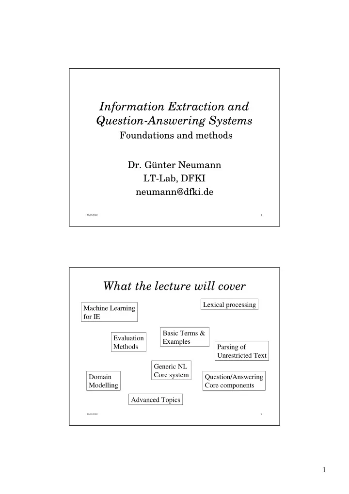
Information Extraction and Question-Answering Systems

Foundations and methods

Dr. Günter Neumann

LT-Lab, DFKI neumann@dfki.de

22/02/2002 2

What the lecture will cover

Basic Terms & Examples Evaluation Methods Generic NL Core system Lexical processing Machine Learning for IE Parsing of Unrestricted Text Domain Modelling Question/Answering Core components Advanced Topics

SLIDE 2

2

22/02/2002 3

POS tagging

Assigning morpho-syntactic categories

to words in context

The green trains run down that track. Det Adj/NN NNS/VBZ NN/VB Prep/Adv/Adj SC/Pron NN/VB Det Adj NNS VB Prep Pron NN

Disambiguation: a combination of lexical

and local contextual constraints

22/02/2002 4

POS tagging

Major goal is to assign/select correct POS

before syntactic analysis

Shallow processing Handling of unknown words (robustness) Reducing search space for next processing stages (parsing)

Good enough for many applications

Information retrieval/extraction Spelling correction Text to speech Terminology extraction/mining

SLIDE 3

3

22/02/2002 5

POS tagging

Corpus approach

NL text for which all correct POS are already assigned Use it as a history for already made disambiguation decisions

Major goal:

extract underlying rules/decisions so that new untagged corpus can be automatically tagged using the extracted rules

22/02/2002 6

POS tagging

Simple method:

pick the most likely tag for each word

The probabilities can be estimated from a tagged corpus Assumes independence between tags Works pretty well (> 90% word tag accuracy) But not good enough for processing of small NL text input: One in ten words wrong

SLIDE 4

4

22/02/2002 7

Simple tagger example

Brown corpus, 1M tagged wrds, 40 tags
Example:

The representatives put the chairs on the table. Word put occurs 41191,

41145 times tagged as VBD 46 times as NN

P(VBD|W=put) = 41145/ 41191 = 0.999 P(NN|W=put) = 46/ 41191 = 0.001

Unknown words:

If w is capitalized then tag(w)=NE else tag(w)=NN

22/02/2002 8

POS problems

Long distance dependencies (findet .... statt),
Annotation errors,
not enough features, e.g., case assignment

(Nom vs. Acc, Er sieht das Haus)

If more features then more data sparseness

problems

Large corpora are needed

SLIDE 5

5

22/02/2002 9

POS corpus approaches

Rule based

Transformation-based error-driven learning (Brill 95) Inductive logic programming (Cussens 97)

Statistical based

Markov models (TnT, Brants 00) Maximum entropy (Ratnaparkhi, 96)

22/02/2002 10

Transformation-based error driven learning (Brill, 95)

Unannotated text Initial state Annotated text learner Truth rules

annoted reference corpus Ordered list of transformation

SLIDE 6

6

22/02/2002 11

Structure of a transformation

Rewrite rule

Change the tag from modal to noun

Triggering environment

The preceding word is a determiner

Application example

The/det can/modal rusted/verb. The/det can/noun rusted/verb.

22/02/2002 12

Generic learning method

At each iteration of learning

Determine transformation t whose application results in the best score according to the objective function used Add t to list of ordered transformations Update training corpus by applying the learned transformation Continue until no transformation can be found whose application results in an improvement to the annoated corpus

Greedy search:

h(n) = estimated cost of the cheapest path from the state represented by the node n to a goal state

best-first search with h as its "eval" function.

SLIDE 7

7

22/02/2002 13

Greedy search

Annotated corpus Err=5100 Annotated corpus Err=3145 Annotated corpus Err=3910 Annotated corpus Err=6300 Annotated corpus Err=3310 Annotated corpus Err=2110 Annotated corpus Err=1231 Annotated corpus Err=4224 Unannotated corpus Annotated Corpus Err=5100 Initial state annotator

T1 T2 T3 T4 T1 T2 T3 T4

22/02/2002 14

Instances of TBL schema

The initial state annotator
Te space/structure of allowable

transformations (patterns)

The objective function for comparing the

corpus to the truth

Applications

Pos tagging PP-attachment Parsing Word sense disambiguation

SLIDE 8

8

22/02/2002 15

TBL POS tagging

Initial annotator (our simple method)

Assign each word its most likely tag Tag unknown words as proper noun if capitalized and common noun otherwise

Error triple: <taga,tagb,number>

Number of times tagger mistagged a word with taga when it should have been tagged with tagb

22/02/2002 16

Transformation patterns

Change tag a to tag b when 1. Preceding (following) word is tagged z 2. The word two before (after) is tagged z 3. One of the two preceeding (following) words is tagged z 4. One of the three preceeding (following) words is tagged z 5. The preceeding word is tagged z and the following word is tagged w 6. The preceeding (following) word is tagged z and the word two before (after) is tagged w Learning task

apply every possible transformation t
count the number of tagging errors caused by t
choose the transformation with the highest error reduction

SLIDE 9

9

22/02/2002 17

Examples of learned transformation from PennWSJ

Next tag is NN DT IN 17 Next tag is VBZ WDT IN 16 ...

Prev. tag is NNS

VBD VBN 7

Prev. tag is PRP

VBD VBN 6 One of the prev. 3 tags is VBZ VBN VBD 5 One of the prev. 2 tags is DT NN VB 4 One of the prev. 2 tags is MD VB NN 3 One of the prev. 3 tags is MD VB VBP 2 Previous tag is TO VB NN 1 Condition To From #

To/TO conflict/NN/VB might/MD vanish/VBP/VB might/MD not reply/NN/VB

22/02/2002 18

Lexicalized transformations

Change tag a to b when

The preceding (following) word is w The word before (after) is w ...

Example (WSJ): wi: word at position i

From IN to RB if wi+2 = as From VBP to VB is (wi-2 or wi-1) = n‘t

SLIDE 10

10

22/02/2002 19

Tagging Performance

97 378 600K TBL W/o Lex. rules 97.2 447 600K TBL With Lex. rules 215 10,000 6,170 # rules or contex. Probs 96,7 64 TBL With Lex. rules 96,7 1M Stochastic 96.3 64K Stochastic Acc. (%) Tagging corpus size (words) Method Closed vocabulary assumption: All possible tags for all words in the test set are known

22/02/2002 20

Handling unkown words

Change the tag of an unknown word (from X)

to Y if

Deleting prefix (suffix) x, |x|≤ 4, results in a (known) word The first (last) 1,2,3,4 characters of the word are x Adding character string x as prefix (suffix) results in a word Word W ever appears immediately to the left (right) of the word Character Z appears in the word

SLIDE 11

11

22/02/2002 21

Some example transformations

... Word it appears to the left VBZ NNS 5 Has suffix -ly RB ?? 4 Has suffix -ed VBN NN 3 Has character . CD NN 2 Has suffix -s NNS NN 1 Condition To From #

Tagging performance: Unknown word accuracy on WSJ test corpus: 82.2% Overall accuracy: 96.6%

22/02/2002 22

Unsupervised TBL

Goal: automatically train a rule-based POS

tagger without using a manually tagged corpus

Source: a dictionary listing the allowable

parts of speech for each word

Challenge: define an objective function for

training that does not need a manually tagged corpus as truth

SLIDE 12

12

22/02/2002 23

Core idea

Note that for ambiguous words we can only

randomly choose between the possible tags

The can will be crushed

Using an unannotated corpus and a

dictionary, we could discover, that of the words that appear after The that have only

ne possible tag, nouns are most common

Change tag of a wrd from (MD|NN|VB) to NN if the previous word is The

22/02/2002 24

Transformation Templates

Change the tag of a word from χ to Y in

context C if:

1. The previous tag is T 2. The previous word is W 3. The next tag is T 4. The next word is W

Different use of transformation: reduce

uncertainty instead of changing one tag to a another ⇒ Y ∈ χ

SLIDE 13

13

22/02/2002 25

Examples of transformations

Change the tag:

From NN|VB|VBP to VBP if the previous tag is NSS From NN|VB to VB if the previous tag is MD From JJ|NNP to JJ if the following tag is NNS

22/02/2002 26

Scoring criterion

Learner has no gold standard training corpus

with which accuracy can be measured

Instead: use information from the distribution
f unambiguous words
Initially, each word in the training corpus is

tagged with all tags allowed for that word

In later learning iterations, training set is

transformed as a result of applying previously learned transformations

SLIDE 14

14

22/02/2002 27

Computation of the score of a tranformation

For each tag Z ∈ χ, Z≠Y, compute freq(Y)/freq(Z)*incontext(Z,C)

freq(Y) = # occurences of words unambiguously tagged with Y; the same for freq(Z) incontext(Z,C) = # times a word unambig. tagged as Z occurs in C

Let: R=argmaxzfreq(Y)/freq(Z)*incontext(Z,C)
Then Change the tag of a word from χ to Y in context C is:

Incontext(Y,C)-freq(y)/freq(R)*incontext(R,C)

Computing the difference between the number of unambiguous

instances of tag Y in context C and the number of unambiguous instances of the most likely tag R in context C, where R∈ χ, R≠Y. Choose the transformation which maximizes this function.

22/02/2002 28

Evaluation results

When tagset of a word not fully

disambiguated, choose randomly a single tag

Results (Training/Test)

PennTB (120K wrds/200T wrds): 95.1%, 1,151 rules learned BrownTB (350T wrds /200T wrds): 96.0%, ~1,729 rules learned

SLIDE 15

15

22/02/2002 29

Final remarks

Weakly supervised rule learning:

Best score: 96.8% using 88,200 corpus (better than supervised on same corpus)

Further issues

Rules can be converted into deterministic FST: O(n), independent of # rules (cf. Roche&Schabes, 1995) Get the source code for free

22/02/2002 30

Main Information Sources for statistical POS Tagging

Paradigmatic information - the distribution of tags

for the word in isolation: P(t|w) P(VBD|W=put) = 41145/ 41191 = 0.999 P(NN|W=put) = 46/ 41191 = 0.001

Syntagmatic information - look at the tags of other

words in the context of the word we are interestd in a new play: AT JJ NN versus AT JJ VBP

SLIDE 16

16

22/02/2002 31

Statistical POS tagging

We would like to have a statistical

model that would be able to take into account both types of information in a principled way

Learn that information from some annotated corpus (i.e., from examples,

bservations)

Keep the syntagmatic context as local as possible

22/02/2002 32

Brief excursion: probability theory (1)

0 ≤ P(A) ≤ 1
P(A+B)= P(A) + P(B), if A & B are independent
P(A+¬A) =P(A) + P(¬ A), ¬ A is the negation of A
P(A) + P(¬ A) = 1

SLIDE 17

17

22/02/2002 33

Brief excursion: probability theory (2)

Let P(A)=k/N, P(B)=l/N,P(AB)=m/N
Then P(B|A) = P(AB)/P(A) = m/k
Chain rule:
Bayes rule:

) ... ( ) ... ( ) ... | (

1 1 1 1 1 1 − − −

=

n n n n n

A A P A A A P A A A P

) ( ) | ( ) ( ) | ( A P B A P B P A B P =

22/02/2002 34

Brief excursion: probability theory (3)

Maximum Likelihood Estimates

) ... ( ) ... ( ) ... | ( ) ... ( ) ... (

1 1 1 1 1 1 1 − −

= =

n n n n MLE n n MLE

W W C W W C W W W P N W W C W W P

SLIDE 18

18

22/02/2002 35

N-Gram Model of Language

Predict a word or properties of a word on the basis
f already observed sequences of words

Morgen gehe ich ins ... (Kino/Theater/...) P(wn|w1,..., wn-1)

Question:

How many words should we look back?

Markov assumption:

Only a few is enough

N-gram: consider a context of length (N-1)

unigram (no context), bigram (previous word), trigram (last previous words)

22/02/2002 36

Markov Models

A system

which may be described at any time as being in one of N distinct states At each discrete time step, the system undergoes a change

f state according to a set of probabilities associated with

the state

Let Q = (q1, ...,qT) be a sequence of random

variables taking values in some finite set S={s1,...,sN}. Markov properties: Limited horizont: a word’s tag only depends on the previous word’s tag (order 1 Markov Model)

P(qt+1=sk| q1, ...,qt)= P(qt+1=sk| qt)

Time invariant: tag probabilities don’t change over time

) | ( ) | ( : ,

1 1 i k t i k t j t i t

s q s q P s q s q P k t = = = = = ∀

− + + −

SLIDE 19

19

22/02/2002 37

Markov Model

i a j i a s q s q P a

N j ij ij i t j t ij

∀ = ∀ ≥ = = =

∑

= +

, 1 , , , ), | (

1 1

Stochastic transition matrix: Markov model as a probabilistic FSA:

N V A

0.25 0.50 0.25

1 ), (

1 1

= = =

∑

= N i i i i

s q P π π

Probs for initial states: 1 1

22/02/2002 38

Hidden Markov Model

Observation/Output is a probabilistic function; doubly

embedded stochastic process 1. Probability of observation (output sequence) 2. Probability of internal process (internal state sequence), which are not observable (hidden); Indirectly observable only through 1.

Thus a HMM λ is characterized by a tripple

(A,B, π), with 1. A, a matrix of transition probabilities 2. B, a matrix of observation (emission) probabilities 3. π, a vector of initial probabilities

SLIDE 20

20

22/02/2002 39

Example HMM

In an HMM, any sequence of states can generate any sequence of observations with a given probability.

  

=

1 7 . 3 . 2 . 5 . 3 . A

  

=

1 5 . 5 . 1 B

  

=

4 . 6 . π

22/02/2002 40

Hidden Markov Models

Prototypical tasks to which HMMs are

applied include the following. Given a sequence of signals O = {o1, ..., on}:

Determine the most probable state sequence that can give rise to this signal sequence. (Viterbi algorithm) Determine the set of model parameters λ = (A,B,

π), maximizing the probability of this signal

sequence. (Baum-Welch algorithm)
Part-of-speech tagging is an example of the

first task and training an HMM is an example of the second.

SLIDE 21

21

22/02/2002 41

HMM (cont.)

Ergodic model: every state of an HMM is

connected with all other states

HMM and POS

Observable sequence: words Hidden sequence: part-of-speech

Thus seen it is assumed that a string α was

generated from some hidden POS sequence; therefore, the major goal is to determine the most probable POS sequence which could have generated α.

22/02/2002 42

Markov Models for POS Tagging

Given a string of words w1,n find a

sequence of tags t1,n that maximizes P(t1,n|w1,n)

Using Bayes Rule:
We need to find t1,n that maximizes the

numerator

) ( ) ( * ) | ( ) | (

, 1 , 1 , 1 , 1 , 1 , 1 n n n n n n

w P t P t w P w t P =

SLIDE 22

22

22/02/2002 43

Example

le/art le/pro gros/adj gros/noun chat/noun

22/02/2002 44

Two main independence assumptions

Words are independent of each other

) | ( * ... * ) | ( * ) | ( ) | (

, 1 , 1 2 , 1 1 , 1 , 1 n n n n n n

t w P t w P t w P t w P =

The probability of a word depends only
n its tag (bigram tagging)

) | ( ) | (

, 1 i i n i

t w P t w P =

SLIDE 23

23

22/02/2002 45

Probability model for P(t1,...,tn)

Breakdown of joint probability:

P(t1,...,tn)= P(tn|t1,...,tn-1)* P(tn-1|t1,...,tn-2)... P(t1)

First order Markov Model:

P(tn|t1,...,tn-1)= P(tn|tn-1)

Thus we get:

P(t1,...,tn)= P(tn|tn-1)* P(tn-1|tn-2)... P(t1)

With a simple Markov model we need to find

the POS sequence P(t1,...,tn) that maximizes

∏ = − n i i i i i t t P t w P 1 1 ) | ( * ) | (

22/02/2002 46

Two main questions

How do we obtain (train) these probabilities?

Calculate estimated probabilities based on frequency counts from a corpus Smooth the estimated probabilities to avoid anomalies due to data sparseness

How do we efficiently find the sequence of the

tags that maximizes the joint product?

Viterbi algorithm

SLIDE 24

24

22/02/2002 47

Maximum Likelihood Estimation

Back to our simple example: The representative put . . .

AT NN VBD/NN

P(VBD|put,NN) = P(put|VBD)P(VBD|NN)

In the training data, we find 41,145 occurrences of put as a verb out of 7,305,323 verbs, so P(put|VBD) = 41145/7305323 = 0.0056

And, out of 4,236,041 occurrences of the tag NN, the tag VBD comes

next 389,612 times: P(VBD|NN) = 389612/4236041 = 0.092

Combining

P(VBD|put,NN) = 41145/7305323 × 389612/4236041 = 0.00052 P(NN|put,NN) = 46/4236041 × 717415/4236041 = 0.0000018

22/02/2002 48

Smoothing of the Probabilities

Data sparseness is always a problem when

estimating probabilities based on a corpus of data

The „adding one'' smoothing technique: add a count
f one to all events, so that there are no zero

probabilities B N w C w P

n n

+ + = 1 ) ( ) (

, 1 , 1

C: absolute frequency of x N: number of training instances B: number of different types

SLIDE 25

25

22/02/2002 49

Smoothing of the Probabilities

Linear interpolation methods can compensate for data sparseness

with higher order models. A common method is interpolating trigrams, bigrams and unigrams:

) | ( ) | ( ) ( ) | (

2 , 1 3 3 1 2 2 1 1 1 , 1 − − − −

+ + =

i i i i i i i i

t t P t t P t P t t P λ λ λ

Usually, the lambda values are automatically determined

using a variant of the Expectation Maximation algorithm.

∑

= ≤ ≤

i i i

1 , 1 λ λ

22/02/2002 50

Pseudo code for viterbi algorithm

Incremental left-to-right search using dynamic programming
δi(j) is the probability of the most likely sequence of tags that ends with

word i having the tag tj

ψi+1(j) gives us the most likely tag at word i given that we are in state j at

word i+1

Induction

Find probability of most likely sequence that ends with word i+1 having tag j, by considering all possible tags for previous word i:

δi+1(j) =max1≤k≤T[δi(k) *P(tj| tk)*P(wí+1| tj)]

For specific tag tk that resulted in the above max, set: ψi+1(j)= tk

Start with δ1(period)=1, δ1(t)=0 for all t ≠ period
At the end find the tag t for which δn+1(t) is the greatest
Reconstruct

the most likely sequence

f

tags by backtracking: X n+1=t, for i=n downto 1 do: Xi= ψi+1(X i+1 )

SLIDE 26

26

22/02/2002 51

Core Idea of Viterbi Algorithm

k aNk

N 1 2 3 4 1 2 t-1 t t+1 T-1 T O1 O2 Ot-1 Ot Ot+1 OT+1 OT a1k time state

bservation

22/02/2002 52

Further Issues with Markov Model Tagging

Unknown words are a problem, since we don't have the

required probabilities. Possible solutions: assign the word probabilities based on corpus-wide distributions of POS use morphological cues (capitalization, endings) to assign a more calculated guess

Using higher order Markov Models:

using a trigram model for POS captures more context and is thus potentially a better probability model However, data sparseness is much more of a problem The Viterbi search for trigrams is more complex

SLIDE 27

27

22/02/2002 53

TnT – Trigrams‘s Tags

Efficient statistical part-of-speech tagger

developed by Thorsten Brants, ANLP-2000

Stochastic models for English (Susanne corpus) and German (Negra corpus) Performance: between 30,000 and 60,000 tokens per second on a Pentium 500 running Linux.

TnT is a trainable tagger (you can use it

with your own annotated corpus)

Home page

http://www.coli.uni-sb.de/~thorsten/tnt/ Online testing of TnT

22/02/2002 54

Example

SLIDE 28

28

22/02/2002 55

Accuracy

96,6% 150,000 Mixed English Susanne Corpus 96,7% 1,200,00 Newspaper English PennTB 96,7% 350,000 Newspaper German NEGRA Corpus Accuracy Size Domain Language Corpus

22/02/2002 56

Underlying Model

Trigram modelling

The probability of a POS only depends on its two preceding POS The probability of a word appearing at a particular position given that its POS occurs at that position is independent of everything else

Explicit consideration of punctuation through special tags

t-1, t0 beginning of sentence tT+1 end of sentence

Tagging is performed by a variant of the Viterbi algorithm

(using beam search)

) | ( ) | ( ) , | (

1 1 2 1 ...

max arg

1

T T T i i i i i i t t

t t P t w P t t t P

T

+ = − −



∏

SLIDE 29

29

22/02/2002 57

Training

Maximum likelihood estimates

) ( ) , ( ) | ( : ) , ( ) , , ( ) , | ( : ) ( ) , ( ) | ( : ) ( ) ( :

3 3 3 3 3 3 2 3 2 1 2 1 3 3 3 2 2 3 3 3

t c t w c t w P Lexical t t c t t t c t t t P Trigrams t c t t c t t P Bigrams N t c t P Unigrams = = = =

Smoothing: context-independent variant of linear

interpolation all trigrams get the same λs ) , | ( ) | ( ) ( ) , | (

2 1 3 3 2 3 2 3 1 2 1 3

t t t P t t P t P t t t P λ λ λ + + =

ˆ ˆ ˆ ˆ

ˆ ˆ ˆ

22/02/2002 58

Smoothing algorithm

Set λi=0
Foreach trigram t1 t2 t3 with f(t1, t2, t3 ) > 0

Depending on the max of the following three values:

Case ( f(t1, t2, t3 )-1 )/ f(t1, t2):

incr λ3 by f(t1, t2, t3 )

Case ( f(t2, t3 )-1 )/ f(t2):

incr λ2 by f(t1, t2, t3 )

Case ( f(t3 )-1 )/ N-1:

incr λ1 by f(t1, t2, t3 )

End

End
Normalize λi
1 means: taking unseen data into account

SLIDE 30

30

22/02/2002 59

Handling of unknown words

Suffix analysis:

The probability distribution for a particular suffix is generated from all words in the training set that share the same suffix Suffix here means „final sequence of characters

f a word“, which is not necessarily

linguistically meaningful

Suffix length in TnT: use the longest suffix

that can be found in the training set (>1)

22/02/2002 60

Suffix estimation

Calculate the probability of a tag t given the last i

letters l of an n letter word

) ,..., ( ) ,..., , ( ) ,..., | ( ˆ

1 1 1 n i n n i n n i n

l l c l l t c l l t P

+ − + − + −

=

) ,..., ( ) ,..., , ( ) ,..., | ( ˆ

1 1 1 n i n n i n n i n

l l c l l t c l l t P

+ − + − + −

=

Smoothing: successive abstraction through sequences
f increasingly more general contexts (i.e., omit more

and more characters of the suffix)

SLIDE 31

31

22/02/2002 61

Evaluation

" Evaluation using two corpora:

NEGRA Corpus: Frankfurter Rundschau (German newspaper texts)
Penn Treebank: Wall Street Journal

" Disjoint training and test parts, 10-fold cross-validation " Tagging accuracy: percentage of correctly assigned tags when assigning

ne tag to each token

" Tagging accuracy depending on the size of the training set " Tagging accuracy depending on the existence of alternative tags

within some beam (reliable vs. unreliable assignments)

22/02/2002 62

Part-of-Speech Tagging with TnT: NEGRA Corpus

Overall Known Unknown min = 78.1% max = 96.7% min = 95.7% max = 97.7% min = 61.2% max = 89.0% NEGRA corpus: 350,000 tokens newspaper text (Frankfurter Rundschau) randomly selected training (variable size) and test parts (30,000 tokens) 10 iterations for each training size; training and test parts are disjoint No other sources were used for training. 1 2 5 10 20 50 100 200 320 50 60 70 80 90 100 Training Size (x 1000)

Avg. % Unknown
Avg. Accuracy

46.4 41.4 36.0 30.7 23.0 18.3

14.3

11.9 50.8

SLIDE 32

32

22/02/2002 63

Part-of-Speech Tagging with TnT: Penn Treebank

Overall Known Unknown min = 78.6% max = 96.7% min = 95.2% max = 97.0% min = 62.2% max = 85.5% Penn Treebank: 1,2 million tokens newspaper text (Wall Street Journal) randomly selected training (variable size) and test parts (100,000 tokens) 10 iterations for each training size; training and test parts are disjoint. No other sources were used for training. 1 2 5 10 20 50 100 200 500 1000 50 60 70 80 90 100

42.8 26.8 20.2 13.2 9.8

7.0

4.4 2.9 50.3

Training Size (x 1000)

Avg. % Unknown
Avg. Accuracy

33.4

22/02/2002 64

Additonal remarks

Procedure of suffix handling is restricted to words

with a certain frequency threshold (< 10)

Capitalization information
Beam search variant of Viterbi algorithm

Instead of considering all possible states during

ne iteration, only consider states whose values

pass a certain predefined threshold θ But note: now, it is not guaranteed that path with the highest probability is found Brants shows that setting θ appropriately doubles performance speed without affecting the accuracy