INF3490 - Biologically inspired computing Unsupervised Learning - PowerPoint PPT Presentation
INF3490 - Biologically inspired computing Unsupervised Learning Weria Khaksar October 24, 2018 Slides mostly from Kyrre Glette and Arjun Chandra training data is labelled (targets provided) targets used as feedback by the algorithm to
INF3490 - Biologically inspired computing Unsupervised Learning Weria Khaksar October 24, 2018
Slides mostly from Kyrre Glette and Arjun Chandra
• training data is labelled (targets provided) • targets used as feedback by the algorithm to guide learning
what if there is data but no targets?
• targets may be hard to obtain / boring to generate Saturn’s moon, Titan https://ai.jpl.nasa.gov/public/papers/hayden_isairas2010_onboard.pdf • targets may just not be known
• unlabeled data • learning without targets • data itself is used by the algorithm to guide learning • spotting similarity between various data points • exploit similarity to cluster similar data points together • automatic classification!
since there is no target , there is no task specific error function
usual practice is to cluster data together via “ competitive learning” e.g. set of neurons fire the neuron that best matches (has highest activation w.r.t.) the data point/input
k-means clustering
• say you know the number of clusters in a data set, but do not know which data point belongs to which cluster • how would you assign a data point to one of the clusters?
• position k centers (or centroids) at random in the data space • assign each data point to the nearest center according to a chosen distance measure • move the centers to the means of the points they represent • iterate
typically euclidean distance x 2 (x 12, x 22 ) √ (x 12 - x 11 ) 2 + (x 22 - x 21 ) 2 x 22 - x 21 (x 11, x 21 ) x 12 - x 11 x 1
k? • k points are used to represent the clustering result, each such point being the mean of a cluster • k must be specified
1) pick a number, k , of cluster centers (at random, do not have to be data points) 2) assign every data point to its nearest cluster center (e.g. using Euclidean distance) 3) move each cluster center to the mean of data points assigned to it 4) repeat steps (2) and (3) until convergence (e.g. change in cluster assignments less than a threshold)
x 1 x 2
x 2 k 1 k 2 k 3 x 1
x 2 k 1 k 2 k 3 x 1
x 2 k 1 k 2 k 3 x 1
x 2 k 1 k 2 k 3 x 1
x 2 k 1 k 2 k 3 x 1
x 2 k 1 k 2 k 3 x 1
x 2 k 1 k 2 k 3 x 1
• results vary depending on initial choice of cluster centers • can be trapped in local minima k 1 • restart with different random centers k 2 • does not handle outliers well
• results vary depending on initial choice of cluster centers • can be trapped in local minima • restart with different k 2 k 1 random centers • does not handle outliers well
let’s look at the dependence on initial choice... x 2 x 1
a solution... x 2 x 1
another solution... x 2 x 1
yet another solution... x 2 x 1
not knowing k leads to further problems! x 2 x 1
not knowing k leads to further problems! x 2 x 1
• there is no externally given error function • the within cluster sum of squared error is what k‐means tries to minimise • so, with k clusters K 1 , K 2 , ..., K k , centers k 1 , k 2 , ..., k k , and data points x j , we effectively minimize:
• run algorithm many times with different values of k • pick k that leads to lowest error without overfitting • run algorithm from many starting points • to avoid local minima
• mean susceptible to outliers (very noisy data) • one idea is to replace mean by median • 1,2,1,2,100? • mean: 21.2 (affected) • median: 2 (not affected) undesirable desirable
• simple : easy to understand and implement • efficient with time complexity O(tkn) n = #data points, k = #clusters, t = #iterations • typically, k and t are small, so considered a linear algorithm
• unable to handle noisy data/outliers • unsuitable for discovering clusters with non-convex shapes • k has to be specified in advance
Example: K‐Means Clustering Example
Some Online tools: Visualizing K‐Means Clustering K‐means clustering
clustering example: evolutionary robotics • 949 robot solutions from simulation • identify a small number of representative shapes for producution
self-organising maps
• high dimensional data hard to understand as is • data visualisation and clustering technique that reduces dimensions of data • reduce dimensions by projecting and displaying the similarities between data points on a 1 or 2 dimensional map
• a SOM is an artificial neural network trained in an unsupervised manner • the network is able to cluster data in a way that topological relationships between data points are preserved • i.e. neurons close together represent data points that are close together
e.g. 1‐D SOM clustering 3‐D RGB data 2‐D SOM clustering 3‐D RGB data #ff0000 #ff1122 #ff1100
• motivated by how visual, auditory, and other sensory information is handled in separate parts of the cerebral cortex in the human brain • sounds that are similar excite neurons that are near to each other • sounds that are very different excite neurons that are a long way off • input feature mapping!
• so the idea is that learning should selectively tune neurons close to each other to respond to/represent a cluster of data points • first described as an ANN by Prof. Teuvo Kohonen
SOM consists of components called nodes/neurons 1,1 each node has a position 2,4 3,3 associated with it on the map 4,5 and a weight vector of dimension given by the data points (input vectors) e.g. say, 5D input vector
feature/output/ map layer and so on... weighted i.e. fully connections connected input layer
neurons are interconnected within a defined neighbourhood (hexagonal here) i.e. neighbourhood relation defined on output layer
typically, rectangular or hexagonal lattice neighbourhood/t opology for 2D SOMs
lattice responds to input j one neuron wins, i.e. has the highest response w j1 (known as the best . . . w jn w j2 w j3 matching unit ) w j4 . . . x n x 1 x 2 x 3 x 4
• input and weight vectors can be matched in numerous ways • typically: Euclidean Manhattan Dot product
adapting weights of winner (and its neighbourhood to a j lesser degree) to closely resemble/match inputs . . . ...and so on for all neighbouring nodes... . . . x 1 x 2 x 3 x 4 x n
j . . . ...and so on with N(i,j) deciding how much to . . . adapt a neighbour’s weight vector x 1 x 2 x 3 x 4 x n
N(i,j) is the neighbourhood function j . . . . . . x 1 x 2 x 3 x 4 x n
N(i,j) tells how close a neuron i is from the winning neuron j j the closer i is from j on the lattice , the higher . . . is N(i,j) . . . x 1 x 2 x 3 x 4 x n
N(i,j) will be rather high i for this neuron! j . . . . . . x 1 x 2 x 3 x 4 x n
but not as high i for this so, update of weight j vector of this neuron will be smaller in other words, this neuron will not be . . . moved as much towards the input , as . . . compared to neurons x 1 x 2 x 3 x 4 x n closer to j
neurons competing to match data point one winning adapting its weights towards data point and bringing lattice neighbours along
• we end up finding weight vectors for all neurons in such a way that adjacent neurons will have similar weight vectors ! • for any input vector, the output of the network will be the neuron whose weight vector best matches the input vector • so, each weight vector of a neuron is the center of the cluster containing all input data points mapped to this neuron
N(i,j) is such that the i neighbourhood of a j winning neuron reduces with time as the learning proceeds . . . the learning rate reduces with time as . . . well x 1 x 2 x 3 x 4 x n
at the beginning of learning the entire lattice could be the j neighbourhood of neuron j weight update for all neurons will happen in this situation
at some point later, this could be the neighbourhood of j j weight update for only the 4 neurons and j will happen
much further on... j weight update for only j will happen typically, N(i,j) is a gaussian function
• competition ‐ finding the best matching unit/winner, given an input vector • cooperation ‐ neurons topologically close to winner get to be part of the win, so as to become sensitive to inputs similar to this input vector • weight adaptation ‐ is how the winner and neighbour’s weights move towards and represent similar input vectors, which are clustered under them
• we determine the size • big network? • each neuron represents each input vector! • not much generalisation! • small network? • too much generalisation! • no differentiation! • try different sizes and pick the best... 63
• quantization error : average distance between each input vector and respective winning neuron • topographic error : proportion of input vectors for which winning and second place neuron are not adjacent in the lattice
Recommend
More recommend
Explore More Topics
Stay informed with curated content and fresh updates.
