Inexact variable metric proximal gradient methods with line-search - PowerPoint PPT Presentation
Inexact variable metric proximal gradient methods with line-search for convex and nonconvex optimization Silvia Bonettini Dipartimento di Scienze Fisiche, Optimization Algorithms and Software Informatiche e Matematiche for Inverse problemS
Inexact variable metric proximal gradient methods with line-search for convex and nonconvex optimization Silvia Bonettini Dipartimento di Scienze Fisiche, Optimization Algorithms and Software Informatiche e Matematiche for Inverse problemS Università di Modena e Reggio Emilia www.oasis.unimore.it Computational Methods for Inverse Problems in Imaging Como, 16-18 July 2018 Silvia Bonettini Inexact variable metric proximal gradient methods CMIPI 2018 1 / 17
Collaborators and main references Joint works with: Marco Prato, Università di Modena e Reggio Emilia Federica Porta, Simone Rebegoldi, Valeria Ruggiero, Università di Ferrara Ignace Loris, Université Libre de Bruxelles Main references: S. B., I. Loris, F . Porta, M. Prato 2016, Variable metric inexact line–search based methods for nonsmooth optimization, SIAM J. Optim. , 26 (2), 891-921 S. B., F. Porta, V. Ruggiero 2016, A variable metric forward–backward method with extrapolation, SIAM J. Sci. Comput., 38 (4), A2558-A2584 S. B., I. Loris, F . Porta, M. Prato, S. Rebegoldi 2017, On the convergence of a line–search base proximal-gradient method for nonconvex optimization, Inverse Probl. , 33 (5), 055005 S. B., S. Rebegoldi, V. Ruggiero, 2018, Inertial variable metric techniques for the inexact forward-backward algorithm, submitted. Silvia Bonettini Inexact variable metric proximal gradient methods CMIPI 2018 2 / 17
A general nonsmooth problem Several optimization problems arising from the Bayesian approach to inverse prob- lems have the following structure x ∈ R n f ( x ) ≡ f 0 ( x ) + f 1 ( x ) , min where: f 0 ( x ) continuously differentiable, possibly nonconvex. usually expressing some kind of data discrepancy f 1 ( x ) convex, possibly nondifferentiable usually expressing regularization Goal: develop a numerical optimization algorithm producing a good approximation of the solution of the minimization problem in few, cheap iterations. Silvia Bonettini Inexact variable metric proximal gradient methods CMIPI 2018 3 / 17
The class of proximal gradient methods Proximal gradient methods, aka forward-backward methods, exploit the smooth- ness of f 0 and the convexity of f 1 in problem x ∈ R n f ( x ) ≡ f 0 ( x ) + f 1 ( x ) , min Definition (Proximal gradient method) Any first order method based on the following two operations: Explicit Forward/Gradient step: computation of the gradient ∇ f 0 ( x ) Implicit Backward/Proximal step: computation of the proximity (or resolvent) operator: x ∈ R n f 1 ( x ) + 1 2 � x − z � 2 prox f 1 ( z ) = arg min Example: If Ω ⊂ R n is a closed convex set, we can define the indicator function � 0 if x ∈ Ω ι Ω ( x ) = ⇒ prox ι Ω ( z ) = Π Ω ( z ) + ∞ otherwise (orthogonal projection onto Ω ). NB: gradient projection methods are special instances of proximal gradient meth- ods. Silvia Bonettini Inexact variable metric proximal gradient methods CMIPI 2018 4 / 17
A basic forward-backward scheme x ( k ) − α k ∇ f 0 ( x ( k ) ) ← Forward step z ( k ) = y ( k ) prox α k f 1 ( z ( k ) ) ← Backward step = y ( k ) − x ( k ) d ( k ) = x ( k ) + λ k d ( k ) x ( k +1) = NB: The steplength parameters α k , λ k ∈ R > 0 , in standard convergence analysis, are related to the Lipschitz constant L of ∇ f 0 ( x ) [Combettes-Wajs 2006], [Com- bettes, Wu, 2014] requiring that α k and/or λ k ≤ C L A motivating problem: nonnegative image restoration from Poisson data n � g i � � x ∈ R n KL ( Hx, g ) min + ρ �∇ x � + ι R n ≥ 0 ( x ) where KL ( t, g ) = log + t i − g i t i � �� � � �� � i =1 f 0 ( x ) f 1 ( x ) either ∇ f 0 is not Lipschitz or L is very large prox f 1 is not available in closed form Silvia Bonettini Inexact variable metric proximal gradient methods CMIPI 2018 5 / 17
A line–search approach We propose to compute λ k with a line–search approach, starting from 1 and back- tracking until a sufficient decrease of the objective function is obtained. Generalized Armijo rule [Tseng, Yun, 2009, Porta, Loris, 2015, B. et al. , 2016] f ( x ( k ) + λ k d ( k ) ) ≤ f ( x ( k ) ) + βλ k h ( k ) ( y ( k ) ) , where β ∈ (0 , 1) and 1 h ( k ) ( y ) = ∇ f 0 ( x ( k ) ) T ( y − x ( k ) ) + 2 α k � y − x ( k ) � 2 + f 1 ( y ) − f 1 ( x ( k ) ) , NB1: We have y ( k ) = prox α k f 1 ( x ( k ) − α k ∇ f 0 ( x ( k ) ) = arg min y ∈ R n h ( k ) ( y ) . Since h ( k ) ( y ( k ) ) < 0 , we obtain a monotone decrease of the objective function. NB2: For f 1 ≡ 0 , dropping the quadratic term we obtain the standard Armijo rule for smooth optimization. Pros: Cons: No need of any Lipschitz assumption Needs the evaluation of the function f at each backtracking loop (usually 1-2 Adaptive selection of λ k (no user per outer iteration). provided parameter) No assumptions on α k , just be bounded above and away from zero. Silvia Bonettini Inexact variable metric proximal gradient methods CMIPI 2018 6 / 17
Inexact computation of the proximity operator (1) Basic idea y ( k ) of y ( k ) by applying an iterative optimization method Compute an approximation ˜ to the minimum problem defining the proximity operator: y ( k ) ≃ y ( k ) = arg min y ∈ R n h ( k ) ( y ) ˜ with an increasing accuracy as k increases. This results in a two loop algorithm and the question now is How to stop the inner iterations to preserve the convergence of the iterates { x ( k ) } to a solution? We need to define a criterion to measure the accuracy of the approximate proximity operator computation. Crucial properties of this criterion: It has to preserve the convergence properties of the whole scheme. It must be based on computable quantities. Borrowing the ideas in [Salzo,Villa,2012], [Villa etal 2013] replace 0 ∈ ∂h ( k ) ( y ( k ) ) with 0 ∈ ∂ ǫ k h ( k ) (˜ y ( k ) ) Silvia Bonettini Inexact variable metric proximal gradient methods CMIPI 2018 7 / 17
Inexact computation of the proximity operator (2) A well defined primal-dual procedure Assume that f 1 ( x ) = g ( Ax ) , A ∈ R m × n (easy generalization to f 1 ( x ) = � p i =1 g i ( A i x ) ). The dual problem of the proximity operator computation is v ∈ R m Ψ ( k ) ( v ) ≡ − 1 2 α k � α k A T v − z ( k ) � 2 − g ∗ ( v ) + C k x ∈ R n h ( k ) ( x ) = max min where g ∗ is the Fenchel convex conjugate of g . If v ( k ) = arg max Ψ ( k ) ( v ) , then y ( k ) = z ( k ) − α k A T v ( k ) . y ( k ) as follows: Compute ˜ apply a maximization method to the dual problem, generating the dual sequence { v ( k,ℓ ) } ℓ ∈ N converging to v ( k ) y ( k,ℓ ) } ℓ ∈ N , with formula compute the corresponding primal sequence { ˜ y ( k,ℓ ) = z ( k ) − α k A T v ( k,ℓ ) ˜ stop the inner iterations when h ( k ) (˜ y ( k,ℓ ) ) − Ψ ( k ) ( v ( k,ℓ ) ) ≤ ǫ k where C with q > 1 prefixed sequence choice k q ǫ k = or ηh ( k ) (˜ y ( k,ℓ ) ) with η ∈ (0 , 1] adaptive choice Silvia Bonettini Inexact variable metric proximal gradient methods CMIPI 2018 8 / 17
Introducing Scaling Add a new parameter, a s.p.d. scaling matrix D k which determines a different metric at each iterate: replace � x � with � x � D k = x T D k x Variable Metric Inexact Line–Search Algorithm (VMILA) x ( k ) − α k D − 1 z ( k ) k ∇ f 0 ( x ( k ) ) ← Scaled Forward step = α k f 1 ( z ( k ) ) ≡ y ( k ) ← Scaled Inexact Backward step y ( k ) prox D k ˜ ≈ y ( k ) − x ( k ) d ( k ) = ˜ x ( k ) + λ k d ( k ) ← Armijo-like line–search x ( k +1) = Silvia Bonettini Inexact variable metric proximal gradient methods CMIPI 2018 9 / 17
Summary of convergence results about VMILA VMILA λ k with line–search + inexact computation of the proximal point with increasing accuracy + α k bounded Convex case Nonconvex case k →∞ Assumption: D k − → I like Assumption: D k has bounded C/k p , p > 1 eigenvalues. Convergence to a Every accumulation point of { x ( k ) } k ∈ Z is a stationary point minimizer (without Lipschitz assumptions on If f satisfies the ∇ f 0 ( x ) ) Kurdyka–Lojasiewicz property and ∇ f 0 is locally Lipschitz, then Convergence rate f ( x ( k ) ) − f ∗ = O (1 /k ) { x ( k ) } k ∈ Z converges to a (proof with Lipschitz stationary point (with exact assumptions on ∇ f 0 ( x ) ) proximal point computation). Block-coordinate version of VMILA proposed in [B., Prato, Rebegoldi, 2018, to appear ]. NB: α k and D k are required only to be bounded ⇒ use them to implement some acceleration strategy. Silvia Bonettini Inexact variable metric proximal gradient methods CMIPI 2018 10 / 17
Recommend
More recommend
Explore More Topics
Stay informed with curated content and fresh updates.
