INEQUALITY CONSTRAINTS Introduction of Slack Variables Consider - - PDF document

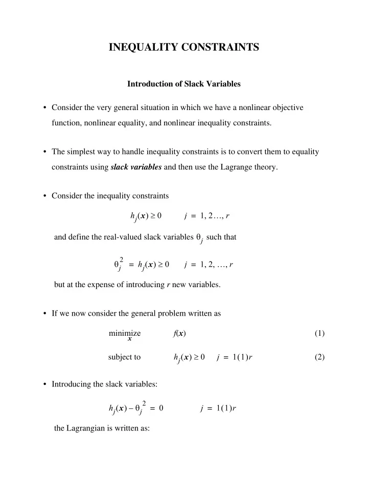
INEQUALITY CONSTRAINTS

Introduction of Slack Variables

• Consider the very general situation in which we have a nonlinear objective

function, nonlinear equality, and nonlinear inequality constraints.

• The simplest way to handle inequality constraints is to convert them to equality

constraints using slack variables and then use the Lagrange theory.

• Consider the inequality constraints

hj x ( ) ≥ j 1 2… r , , = and define the real-valued slack variables θj such that θj

2

hj x ( ) ≥ = j 1 2 … r , , , = but at the expense of introducing r new variables.

• If we now consider the general problem written as

minimize

x

f x ( ) (1) subject to hj x ( ) ≥ j 1 1 ( )r = (2)

• Introducing the slack variables:

hj x ( ) θj

2

– = j 1 1 ( )r = the Lagrangian is written as:

L x λ θ , , ( ) f x ( ) λj hj x ( ) θj

2

– ( )

j 1 = r

∑

+ = (3)

• The necessary conditions for an optimum are:

xi ∂ ∂L xi ∂ ∂f λj xi ∂ ∂hj

j 1 = r

∑

+

x x* = λ λ

*

=

= = i 1 1 ( )n = λj ∂ ∂L hj x ( ) θj

2

–

x x* = θ θ

*

=

= = j 1 1 ( )r = θj ∂ ∂L 2λj

*θj *

– = = j 1 1 ( )r = (4) (5) (6)

• From the last expression (6), it is obvious that either λ* = 0 or θj

*

=

• r both.
• Case 1: λj

*

= , θj

*

≠ In this case, the constraint hj x ( ) ≥ is ignored since hj x* ( ) θj

*

( )

2

> = (i.e. the constraint is not binding). If all λj

*

= , then (4) implies that ∇f x* ( ) = which means that the the solution is the unconstrained minimum.

• Case 2: θj

*

= , λj

*

≠ In this case, we have hj x* ( ) = which means that the optimal solution is on the boundary of the jth constraint. Since λj

*

≠ this implies that ∇f x* ( ) ≠ and therefore we are not at the unconstrained minimum.

• Case 3: θj

*

= and λj

*

= for all j. In this case, we have hj x* ( ) = for all j and ∇f x* ( ) = . Therefore, the boundary passes through the unconstrained optimum which is also the constrained optimum. Example: Now consider the problem minimize

x

f x ( ) x a – ( )2 b + = subject to: x c ≥

b a x

f x ( )

c

f x ( ) x a – ( )2 b + = x c ≥ Sketch of the constrained one dimensional problem.

• The location of the minimum depends on whether or not the unconstrained

minimum is inside the feasible region or not.

• If c

a > then the minimum lies at x c = , which is the boundary of the feasible reagion defined by x c ≥ .

• If c

a ≤ then the minimum lies at the unconstrained minimum, x a = .

• Introducing a single slack variable, θ2

x c – = ≥ : x c – θ2 – = and we can write the Lagrangian as L x λ θ , , ( ) x a – ( )2 b λ x c – θ2 – ( ) + + = where λ is the Lagrange multiplier. x ∂ ∂L 2 x* a – ( ) λ* + = = λ ∂ ∂L x* c – θ* 2 – = = θ ∂ ∂L 2λ* θ* – = = (7) (8) (9)

• In general, we need to know how c and a compare.

• Case 1:

From (9), assume λ* = , θ* ≠ . Therefore, from (7) x* a = and thus from (8), a c – θ* 2 – = which gives that θ* 2 a c – = and we have that θ* is real only for c a ≤ . Now since λ* = we have L x* λ* θ* , , ( ) f x* ( ) =

and x

∂ ∂f

x*

= This tells us that the unconstrained minimum is the constrained minimum.

• Case 2: Now let us assume that λ*

≠ , θ* = . From (8) we have x* c = and from (7) λ* 2 a c – ( ) = . Since λ* ≠ and in the previous case we had c a ≤ , now we have c a > .

• Case 3: For the case λ*

θ* = = , (7) tells us that x* a – = and therefore x* a = . From (8) we have x c – = and therefore x* a c = = . The uncostrained minimum lies on the boundary since from (7) x ∂ ∂L

x*

x ∂ ∂f

x*

= = .

Example: As a two dimensional example, consider minimize

x

f x ( ) x1 3 – ( )2 2 x2 5 – ( )2 + = subject to: g x ( ) 2x1 3x2 5 ≤ – + =

3 6 2 4 6

x2 x1 g 2x1 3x2 5 – + = f x ( ) x1 3 – ( )2 2 x2 5 – ( )2 + = Contours and feasible region for the example problem.

• Unless one was to draw a very accurate contour plot, it is hard to find the

minimum from such a graphical method.

• It is obvious from the graph though, that the minimum will lie on the line

g x ( ) = .

• We introduce a single slack variable, θ2, and construct the Lagrangian as

L x λ θ , , ( ) x1 3 – ( )2 2 x2 5 – ( )2 λ 2x1 3x2 5 θ2 + – + ( ) + + = .

• The inequality constraint was changed to the equality constraint g x

( ) θ2 + = , using the slack variable θ2 g x ( ) – = ≥ .

• The necessary conditions become

x1 ∂ ∂L 2 x1

*

3 – ( ) 2λ* + = = x2 ∂ ∂L 4 x2

*

5 – ( ) 3λ* + = = θ ∂ ∂L 2θ* λ* = = λ ∂ ∂L 2x1

*

3x2

*

5 – θ* 2 + + = = (10) (11) (12) (13) From (10) and (11): x1

*

3 λ* – = x2

*

5 3 4

• λ*

– = substituting these expressions in (13) we have: 2 3 λ* – ( ) 3 5 3 4

• λ*

– ⎝ ⎠ ⎛ ⎞ 5 – θ* 2 + + = 16 17 4

• λ*

θ* 2 + – =

.

If λ* = then θ* will be complex. If θ* = then λ* 64 17 ⁄ = and therefore x1

*

13 17

• –

= x2

*

37 17

• =

θ* = means there is no slack in the constraint as expected from the plot.

The Kuhn-Tucker Theorem

• Kuhn-Tucker theorem gives the necessary conditions for optimum of a nonlinear
• bjective function constrained by a set of nonlinear inequality constraints.
• The general problem is written as

minimize

x

f x ( )

x

n ∈ subject to: gi x ( ) ≤ i 1 2 …r , , = If we had equality constraints, then we could introduce two inequality constraints in place of it. For instance if it was required that h x ( ) = , then we could just impose h x ( ) ≤ and h x ( ) ≥

• r h x

( ) – ≤ .

• Now assume that f x

( ) and gi x ( ) are differentiable functions; The Lagrangian is: L x λ , ( ) f x ( ) λi

i 1 = r

∑

gi x ( ) + = The necessary conditions for x* to be the solution to the above problem are: xj ∂ ∂ f x* ( ) λi

*

xj ∂ ∂ gi x* ( )

i 1 = r

∑

+ = j 1 2 … n , , , = gi x* ( ) ≤ i 1 1 ( )r = λi

* gi x*

( ) = i 1 1 ( )r = λi

*

≥ i 1 1 ( )r = (14) (15) (16) (17)

• These are known as the Kuhn-Tucker stationary conditions; written compactly

as: ∇x L x* λ* , ( ) = ∇λ L x* λ* , ( ) g x* ( ) = ≤ λ* ( )

T

g x* ( ) = λ* ≥ (18) (19) (20) (21)

• If our problem is one of maximization instead of minimization then

maximize

x

f x ( )

x

n ∈ subject to: gi x ( ) ≤ i 1 2 …r , , = we can replace f x ( ) by f x ( ) – in the first condition xj ∂ ∂ f x* ( ) – λi

*

xj ∂ ∂ gi x* ( )

i 1 = r

∑

+ = j 1 2 … n , , , = xj ∂ ∂ f x* ( ) λ – i

*

( ) xj ∂ ∂ gi x* ( )

i 1 = r

∑

+ = j 1 2 … n , , , = (22) . (23)

• For the maximization problem is one of changing the sign of λi

* :

∇x L x* λ* , ( ) = ∇λ L x* λ* , ( ) g x* ( ) = ≤ λ* ( )

T

g x* ( ) = (24) (25) (26)

λ* ≤ (27)

Transformation via the Penalty Method

• The Kuhn-Tucker necessary conditions give us a theoretical framework for

dealing with nonlinear optimization

• From a practical computer algorithm point of view we are not much further than

we were when we started.

• We require practical methods of solving problems of the form:

minimize

x

f x ( ) x n ∈ (28) subject to gj x ( ) ≤ j 1 1 ( )J = hk x ( ) = k 1 1 ( )K = (29) (30)

• We introduce a new objective function called the penalty function

P x R ; ( ) f x ( ) Ω R g x ( ) h x ( ) , , ( ) + = where the vector R contains the penalty parameters and Ω R g x ( ) h x ( ) , , ( ) is the penalty term.

• The penalty term is a function of R and the constraint functions, g x

( ) h x ( ) , .

• The purpose of the addition of this term to the objective function is to penalize

the objective function when a set of decision variables, x, which are not feasible are chosen.

Use of a parabolic penalty term

• Consider the minimization of an objective function, f x

( ) with equality constraints, h x ( ).

• We create a penalty function by adding a positive coefficient times each

constraint, that is minimize

x

P x R ; ( ) f x ( ) Rk hk x ( ) { }2

k 1 = K

∑

+ = . (31) As the penalty parameters Rk ∞ → , more weight is attached to satisfying the kth constraint. If a specific parameter is chosen as zero, say Rk = , then the kth equality constraint is ignored. The user specifies value of Rk according to the importance of satisfying each equality constraint. Example: minimize

x

x2

1

x2

2

+ subject to: x2 1 = We construct a penalty function as: P x R ; ( ) x2

1

x2

2

R x2 1 – ( )2 + + = and we proceed to minimizing P x R ; ( ) for particular values of R.

• We proceed analytically; first order necessary conditions for a minimum

x1 ∂ ∂P 2x1

*

= = x1

*

⇒ = x2 ∂ ∂P 2x2

*

2R x2

*

1 – ( ) + = = x2

*

⇒ R 1 R +

• =

If we now take the limit as R ∞ → , we have x2

*

R 1 R +

• R

∞ →

lim 1 = =

.

• In a numerical procedure, the value of the R would be increased gradually and

the numerical optimization would be performed several times. x2 R ∞ = R 1 =

unconstrained minimum

R = x2 1 = x1 R 2 = Example of the use of a parabolic penalty function.

Inequality constrained problems

• Consider the penalty method for inequality constrained problems.
• The general nonlinear objective function with J nonlinear inequality constraints

is written as minimize

x

f x ( ) x Rn ∈ (32) subject to gj x ( ) ≤ j 1 1 ( )J = (33) A penalty function can be constructed as P x R ; ( ) f x ( ) Ri

i 1 = J

∑

gi x ( ) [ ]2u gi ( ) + = (34) where u gi ( ) is the step-function defined by u gi ( ) if gi x ( ) ≤ 1 if gi x ( ) > ⎩ ⎨ ⎧ = (35) and the penalty parameter is chosen as a positive number, Ri > .

• The term gi x

( ) [ ]2u gi ( ) is sometimes called the bracket operator and is denoted gi x ( ) 〈 〉

• The step-function is used to ignore the constraint when it is satisfied by the

decision variables and to treat it as a penalty term when it is not satisfied.

• When this type of penalty term is used, the method is referred to as an exterior

penalty method since points outside the feasible region are allowed, but are penalized.

• As the penalty parameter increases, the feasibility region is “pushed in”.

gi Ri

violated constraint satisfied

Ω Ri

i 1 = J

∑

gi x ( ) [ ]2u gi ( ) =

constraint 1

Exterior penalty method. Inverse penalty term

• An alternate method which is commonly used is the inverse penaly method.
• If we have a nonlinear optimization problem written as

minimize

x

f x ( ) x Rn ∈ (36) subject to gj x ( ) ≥ j 1 1 ( )J = (37) then we can construct a penalty function as P x R ; ( ) f x ( ) R 1 gi x ( )

• i

1 = J

∑

+ = where only one penalty parameter is used.

• The method is easy to visualize if we consider the case of only one constraint,

J 1 = . Then the penalty term is simply Ω R g x ( )

• =

where g x ( ) is the single constraint.

R

• R

g x ( ) Ω R g x ( )

• =

1

• 1

Inverse penalty term.

• As can be deduced from the figure, it is important that only feasible points be

started with; because of this, this method is classified as an interior method.

• With exterior penalties the parameter R is steadily increased with R

∞ → in the limit so as to exclude infeasible points.

• With interior penalties, the parameter R is steadily decreased with R

→ in the

• limit. Otherwise, you may artificially exclude a minimum located on the

boundary.

Example: In the following problem, solve it using both an interior and exterior method. minimize

x

f x ( ) x1 4 – ( )2 x2 4 – ( )2 + = subject to: g x ( ) 5 x1 x2 ≥ – – = solve using the “bracket operator” P x R ; ( ) f x ( ) R g x ( ) [ ]2u g x ( ) – ( ) + = we have P x R ; ( ) x1 4 – ( )2 x2 4 – ( )2 R 5 x1 x2 – – ( )2u g x ( ) – ( ) + + =

• Thus, when g x

( ) < , i.e. the decision variables are infeasible, then a penalty of R 5 x1 x2 – – ( )2 is applied.

• Proceeding analytically to find the necessary conditions for a minimum, we have

x1 ∂ ∂P 2 x1

*

4 – ( ) 2R ( ) 5 x1

*

x2

*

– – ( ) 1 – ( ) + = = x2 ∂ ∂P 2 x2

*

4 – ( ) 2R ( ) 5 x1

*

x2

*

– – ( ) 1 – ( ) + = = subtracting these two equations 2 x1

*

4 – ( ) 2 x2

*

4 – ( ) – x1

*

⇒ x2

*

= =

.

From the first above, we get x1 4 – ( ) R 5 2x1 – ( ) – = and therefore

x1 5R 4 + 2R 1 +

• =
• Increasing the penalty parameter to ∞, we have

x1

R ∞ →

lim 5 2

• =

and the constrained minimum is: x* 5 2

• 5

2

• ,

⎝ ⎠ ⎛ ⎞ = Since the constraint, g x* ( ) = this implies that the constaint is tight. The unconstrained minimum is at x 4 4 , ( ) = .

• Now solve using the inverse penalty:

P x R ; ( ) f x ( ) R g x ( ) [ ] 1

–

+ = we have P x R ; ( ) x1 4 – ( )2 x2 4 – ( )2 R 5 x1 x2 – – ( ) 1

–

+ + = Whether or not g x ( ) < , i.e. whether or not the decision variables are infeasible, a penalty of R 5 x1 x2 – – ( ) 1

– is applied.

• We must make sure that we remain feasible during the execution of any

algorithm we may employ.

• Proceeding analytically to find the necessary conditions for a minimum, we have

x1 ∂ ∂P 2 x1

*

4 – ( ) R 5 x1

*

x2

*

– – ( )

2

• +

= = x2 ∂ ∂P 2 x2

*

4 – ( ) R 5 x1

*

x2

*

– – ( )

2

• +

= = subtracting these two equations, we again get x1

*

x2

*

= and we also have 4 x1

*

( )

3

36 x1

*

( )

2

– 105x1

*

100 – R 2

• +

+ =

• This equation can be solved, for its roots, and the minimum of P x R

; ( ) for particular values of R can be found. Minimum for different values of R R x1

* x2 *

, f x* ( ) 100 0.5864 23.3053 10 1.7540 10.0890 1 2.2340 6.32375 0.1 2.4113 5.0479 0.01 2.4714 4.6732 0.001 2.4909 4.5548 2.5000 4.5000

• For each value of the penalty parameter, an unconstrained optimization problem

must be solved.