Inclusion of the sorption hysteresis phenomenon in future drying - - PDF document

’The Future of Quality Control for Wood & Wood Products’, 4-7th May 2010, Edinburgh The Final Conference of COST Action E53

Inclusion of the sorption hysteresis phenomenon in future drying models. Some basic considerations.

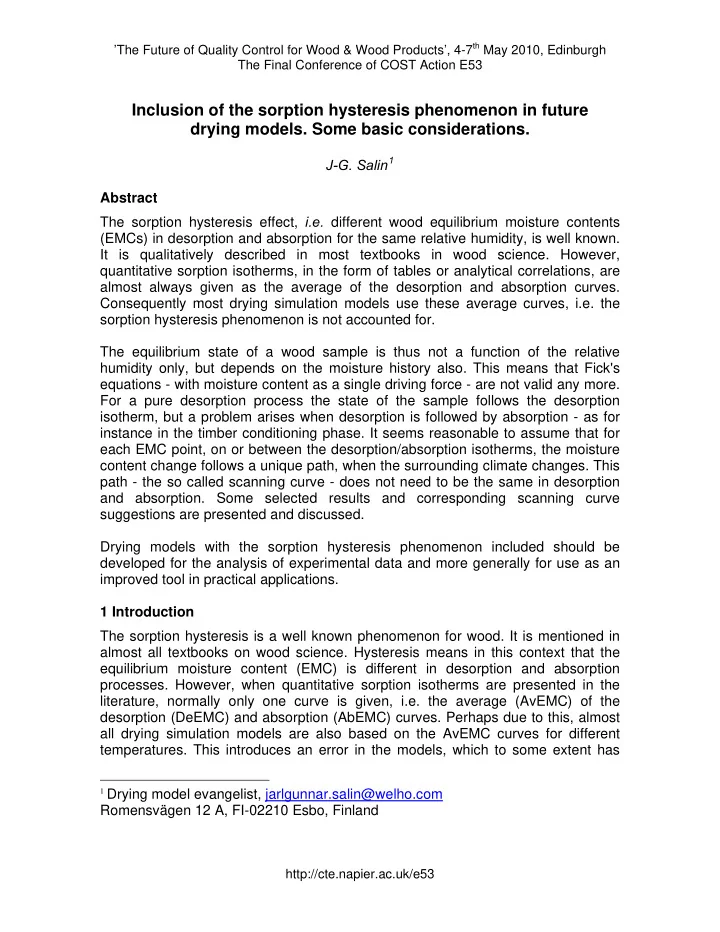
J-G. Salin1 Abstract The sorption hysteresis effect, i.e. different wood equilibrium moisture contents (EMCs) in desorption and absorption for the same relative humidity, is well known. It is qualitatively described in most textbooks in wood science. However, quantitative sorption isotherms, in the form of tables or analytical correlations, are almost always given as the average of the desorption and absorption curves. Consequently most drying simulation models use these average curves, i.e. the sorption hysteresis phenomenon is not accounted for. The equilibrium state of a wood sample is thus not a function of the relative humidity only, but depends on the moisture history also. This means that Fick's equations - with moisture content as a single driving force - are not valid any more. For a pure desorption process the state of the sample follows the desorption isotherm, but a problem arises when desorption is followed by absorption - as for instance in the timber conditioning phase. It seems reasonable to assume that for each EMC point, on or between the desorption/absorption isotherms, the moisture content change follows a unique path, when the surrounding climate changes. This path - the so called scanning curve - does not need to be the same in desorption and absorption. Some selected results and corresponding scanning curve suggestions are presented and discussed. Drying models with the sorption hysteresis phenomenon included should be developed for the analysis of experimental data and more generally for use as an improved tool in practical applications. 1 Introduction The sorption hysteresis is a well known phenomenon for wood. It is mentioned in almost all textbooks on wood science. Hysteresis means in this context that the equilibrium moisture content (EMC) is different in desorption and absorption

• processes. However, when quantitative sorption isotherms are presented in the

literature, normally only one curve is given, i.e. the average (AvEMC) of the desorption (DeEMC) and absorption (AbEMC) curves. Perhaps due to this, almost all drying simulation models are also based on the AvEMC curves for different

• temperatures. This introduces an error in the models, which to some extent has

1 Drying model evangelist, jarlgunnar.salin@welho.com

Romensvägen 12 A, FI-02210 Esbo, Finland

http://cte.napier.ac.uk/e53

’The Future of Quality Control for Wood & Wood Products’, 4-7th May 2010, Edinburgh The Final Conference of COST Action E53

been handled by introducing correction factors. In the following the need to include the sorption hysteresis phenomenon in model work is discussed. After that some problems and solutions in connection with such a model extension are presented. 2 Is the sorption hysteresis important in modelling? The interaction between a piece of wood and the surrounding climate (air temperature and humidity) is of course one of the two main parts in all drying

• models. The other part is the moisture migration inside the wood. The external

interaction includes transfer of heat (energy) as well as moisture (mass) to and from the wood surface. The heat and mass transfer are expressed with the following equations. ) (

s

T T A − = Φ

∞

α Equation 1 ) (

∞

− = c c A m

s

β

• Equation 2

Φ/A = heat flux per unit area (W/m2) α = heat transfer coefficient (W/m2/K) T∞ , Ts = temperature of surrounding air and wood surface, resp. (K) A m

• = moisture flux per unit area (kg/m2/s)

β = mass transfer coefficient (m/s) c∞ , cs = vapour concentration of surrounding air and in equilibrium with the wood surface, resp. (kg/m3) Vapour concentration is here used as the driving force in Equation 2, but it can be discussed whether partial pressure would be a better choice. Anyway, cs is here the point where the sorption curve enters, as it gives the connection between surface moisture content (MC) and the vapour concentration in the air in equilibrium with the surface. For a pure drying process the DeEMC curve should be used for determination of this connection. As the transfer of both heat and moisture occurs through the same air-side boundary layer, it seems reasonable that there should be a coupling between the transfer coefficients α and β. This is referred to as the analogy between heat and mass transfer, which with a good approximation can be expressed as: ρ c β α

p

= Equation 3 where cpρ is the volumetric heat capacity of the humid air in the boundary layer. Equation 3 is important as the mass transfer coefficient can be determined from the heat transfer coefficient which normally is more easily predicted. However,

http://cte.napier.ac.uk/e53

’The Future of Quality Control for Wood & Wood Products’, 4-7th May 2010, Edinburgh The Final Conference of COST Action E53

when drying model simulations have been compared with experimental data, it has frequently been found that Equation 3 seems to overestimate the mass transfer coefficient (Salin 2007). As Equation 3 represents a fundamental relation, this deviation was for a long time not fully understood and correction factors were introduced into the models. However, it seems now that the deviation can be explained by the fact that these models used the AvEMC sorption curves. This is illustrated by Figure 1.

5 10 15 20 25 0,5 Relative humidity Moisture content, % 1

B C A

Figure 1: Example of a drying process in a sorption diagram where A represents the RH of the air and B the MC of the wood surface. In models the RH determined by the average sorption curve (C) is however often used. The curves are, from the top, desorption (DeEMC) average (AvEMC) and absorption (AbEMC) curves. In Figure 1 the real driving force (in a pure drying process) is represented by the distance A-B, which is shorter than the distance A-C used in the model. The correction factor needed is then AB/AC. As seen the correction factor becomes more important when the points B and C are close to the point A. This is in agreement with experimental findings regarding the correction factor. In theory the factor can even be negative. It is further noticed that the correction factor is not a pure wood property, as it is dependent on the relative humidity (RH) of the surrounding air also. (RH is not a physically correct driving force, but as sorption diagrams traditionally use RH as a variable, it is used here for the purpose of illustration only.) It seems that the use of AvEMC sorption curves instead of DeEMC curves in drying processes explain the observed deviations from the analogy between heat and mass transfer (Salin 2007 p.195). As it has turned out to be necessary to use correction factors in this context in present models, a much more reasonable solution would be to include the sorption hysteresis phenomenon directly in future models.

http://cte.napier.ac.uk/e53

’The Future of Quality Control for Wood & Wood Products’, 4-7th May 2010, Edinburgh The Final Conference of COST Action E53

In drying of timber at sawmills, the distance A-B in Figure 1 is normally relatively long, as a rapid drying is preferred. For wooden material in buildings – both indoors and outdoors – the climate variation is normally much smaller and changes frequently from absorption to desorption and vice versa. As noticed above, the correction factor becomes more important when the points A, B and C are close to each other. This means that the sorption hysteresis phenomenon becomes especially important in such building applications. It can be argued that for pure drying processes it is sufficient to use the DeEMC sorption curves instead of the AvEMC curves. However, nowadays the drying process is frequently ended with an equalisation and conditioning phase, which normally means that at least the wood surface will absorb moisture. If so, the error is ‘doubled’ in this part. For big batch kilns it may also occur that timber on the leeward side absorbs moisture just after a fan reversal. Based on these arguments, there is definitely a need to include the sorption hysteresis phenomenon in future drying models and as well in models for the interaction between climate and wood in buildings. Why has this not been done earlier? One reason is certainly that it is a more complicated issue than it may seem at first hand. Some of the main problems will be discussed in the following. 3 Modelling sorption hysteresis One important feature that is introduced when sorption hysteresis is included in the model is illustrated by the following imagined experiment. Consider a completely dry stick of wood. One end of the stick is dipped into water for a moment and the MC in the end increases to, let’s say, 20 %. After that the stick is stored in a climate corresponding to an AvEMC of 10 %. The dry end MC will then gradually approach 10 % but will stop at about 9 % due to the hysteresis effect (AbEMC ~9 %). In the same way the wet end of the stick will also approach 10 % but stops at about 11 % as DeEMC ~11 %. This situation is illustrated in Figure 2. The interesting question is now; will there be a bound water migration from the higher MC towards the lower MC?

Bound water migration driving force? Climate corresponding to AvEMC = 10 % Absorption Desorption MC = 9 % MC = 11 %

Figure 2: Imagined experiment to describe the bound water driving force problem.

http://cte.napier.ac.uk/e53

’The Future of Quality Control for Wood & Wood Products’, 4-7th May 2010, Edinburgh The Final Conference of COST Action E53

As both ends of the stick are in thermodynamic equilibrium with the same climate, they should be in mutual equilibrium also, i.e. no moisture migration should occur. This shows that Fick’s law with MC (or any other ‘moisture concentration in wood’ variable) is not valid any more when sorption hysteresis is taken into account. The state of the wood is not defined by the MC alone, but depends also on how this MC has been reached, i.e. the history of its moisture changes. This means that the driving force for bound water migration has to be changed. The logical solution is to use the state of the air in equilibrium with the wood as the driving force. This idea was suggested already 30 years ago by (Bramhall 1979) who proposed vapour partial pressure as driving force and by (Kawai et al 1978 and Stanish 1986) that proposed chemical potential as driving force. In addition to this change of driving force, it has to be established how the state point of the wood changes, i.e. in which direction will the state move, expressed as a point on or between the DeEMC and AbEMC curves. This is discussed later on. In this context another, rather similar, imagined experiment may be presented. Consider now a thin wood stick initially with an MC corresponding to the fibre saturation point (FSP). One end is dipped into water for a relatively long time so that this becomes completely saturated with water, i.e. an MC in the range 120-250 % depending on wood density. Will there now be a flow of moisture from the very wet end towards the FSP (MC ~30 %) in the other end? Certainly, a flow

• f free water will occur due to capillary forces. The saturated end is in equilibrium

with 100 % RH as there is free water at the surface. This proves that wood with an MC corresponding to FSP is not in equilibrium with 100 % RH, which however

• ften is inaccurately stated. In addition many textbooks and handbooks present

diagrams and tables where an EMC of about 30 % is given for 100 % RH. Kelvin’s law that states that the vapour pressure above a curved liquid surface (meniscus) is lower than above a flat surface is important in this context. This imagined experiment brings of course the focus on the definition of the FSP. Equilibrium with 100 % RH is thus not a useful definition. In the authors opinion, the most useful FSP definition is the point when the cell wall is water saturated but with no free water present. It is generally accepted that several mechanical wood properties – shrinkage/swelling, MOE, MOR, mechano- sorptive creep, etc. – depend on the amount of bound water but not on the amount

• f free water. There may be a transition zone and not a well defined transition

point, but as these mechanical properties are very important for drying induced stress development as well as for shape deformations etc., this definition seems

• appropriate. Experimental determination of FSP values according to this definition

constitutes a problem (as with many other FSP definitions). In addition modelling moisture migration just below or above FSP is still a problem. From a drying modelling point of view it seems logical to extrapolate experimental sorption curves towards 100 % RH – using one of the many sorption models suggested in the literature (Vidal & Cloutier 2005) – and define this point as “EMC for 100 % RH”. In addition Kelvin’s law should be neglected above FSP. However, it is not given that

http://cte.napier.ac.uk/e53

’The Future of Quality Control for Wood & Wood Products’, 4-7th May 2010, Edinburgh The Final Conference of COST Action E53

extrapolation of the DeEMC and AbEMC curves give the same FSP value, and this constitutes still a problem in the modelling procedure. Finally an interesting detail related to the EMC should be mentioned. In textbooks the EMC is normally defined as the MC which a piece of wood gradually attains when stored in a certain climate. (It is in most cases not mentioned that the result depends on the starting point of the state of the wood – see Section 4 on Scanning curves.) It is then implied that the climate is not affected by the moisture flow to or from the sample. But there is another alternative to determine the EMC. If the sample is put into a small compartment, then the climate (air RH) will gradually attain equilibrium with the sample and an EMC situation is the result in this case

• also. This method has actually been used for certain materials to indirectly

determine the MC by measuring the RH in the compartment. In this case it is assumed that the moisture flow to or from the sample can be neglected in comparison with the total wood moisture, i.e. MC is not changed. Again, the result is not depending only on the sample MC, but also on how this MC has been attained (Section 4). An immediate question is whether these two alternatives represent the same basic EMC definition. It is perhaps not a priori self-evident, but by considering an intermediate situation where both air RH and sample MC change towards a mutual equilibrium, it is obviously correct. One should however be careful when comparing desorption from the wood and absorption by the air (and vice versa). This is illustrated by the following example. Consider a cell wall that separates two air volumes (lumina) and that both the air and the wall are initially completely dry. Increase the RH on the ‘left hand side’ of the wall to a constant value. Then the wall absorbs moisture and the MC is increasing. Eventually the air RH on the ‘right hand side’ will start to increase as moisture is transferred through the wall. What will the final RH be? The air absorbs moisture from the cell wall, which looks like the wall would be in a desorption state and the air would follow the DeEMC curve, i.e. approach a lower RH on the ‘right hand side’. But the cell wall MC is continuously increasing, i.e. the wall is actually in an absorption state and thus the AbEMC curve is followed and the RH will finally be the same on both sides. Both the wall and the ‘right hand side’ air are absorbing moisture, although there is a moisture flow from the wall to the air. It should be kept in mind that the hysteresis phenomenon concerns the wood, not the air. Finally a surprising experimental result should be mentioned. There are indications that the EMC and the hysteresis effect are dependent on the sample size (Shmulsky et al 2001). It is known from both experimental results and theoretical principles, that mechanical stress in the wood will influence the EMC. This has been suggested as an explanation, as very small samples should be free of stress. This is in the author’s opinion not a very convincing explanation as tensile stress in the sample should be balanced by compression stress elsewhere – in the absence

• f external forces. Anyway, such phenomena have to be investigated further.

http://cte.napier.ac.uk/e53

’The Future of Quality Control for Wood & Wood Products’, 4-7th May 2010, Edinburgh The Final Conference of COST Action E53

4 Scanning curves For a hygroscopic material without sorption hysteresis, the state of the material will follow a single curve upon changes in the surrounding climate. For wood the situation is more complicated. In a pure drying process the state of the wood follows the desorption curve – but if the climate changes to an absorption situation, then the state point will leave the desorption curve and move towards the absorption curve. The question is now, along which transition curve will the point move? This transition curve is often called a scanning curve. One reasonable first approximation is to assume that the scanning curve is a nearly horizontal straight line between the boundary curves, as illustrated by the A-B-C-D sequence in the upper part of Figure 3. This was for instance proposed by (Time 1998) but she suggested also that a sloping curve, as in the lower part of Figure 3, would reflect the real situation better.

Relative humidity Moisture content, % A B C D

Figure 3: Examples of scanning curve alternatives. In (Frandsen 2007) the behaviour is investigated further. It is assumed that for each point on or between the DeEMC and AbEMC boundary curves, there is a single scanning curve in the desorption direction and a single curve in the absorption direction (not necessarily the same curve). This means that it doesn’t matter how this point has been reached, i.e. it is assumed that history has not any influence at this stage. Based on measurements found in the literature (Frandsen 2007) proposes rather complicated expressions for the scanning curves. These expressions have no physical background, but are chosen to fit experimental data

• nly. Examples of scanning curves are presented in Figure 4 (absorption) and

Figure 5 (desorption) calculated using the parameter values proposed. It is seen in Figures 4 and 5 that these scanning curves are far from horizontal. Further a curve that starts from, for instance, the DeEMC boundary curve will approach the AbEMC boundary curve but never reach it and the same applies in the other direction too.

http://cte.napier.ac.uk/e53

’The Future of Quality Control for Wood & Wood Products’, 4-7th May 2010, Edinburgh The Final Conference of COST Action E53

5 10 15 20 25 0,1 0,2 0,3 0,4 0,5 0,6 0,7 0,8 0,9 1

Relative humidity Moisture content, %

Figure 4: Example of absorption scanning curves according to (Frandsen 2007).

5 10 15 20 25 0,1 0,2 0,3 0,4 0,5 0,6 0,7 0,8 0,9 1

Relative humidity Moisture content, %

Figure 5: Examples of desorption scanning curves according to (Frandsen 2007). The scanning curve model proposed by (Frandsen 2007) is relatively easily implemented in drying simulation software. Other scanning curve models have been suggested, for instance by (Peralta 1995) using the ‘independent-domain theory’, but this model is much more difficult to implement in simulations. As the amount of experimental data in this field is rather limited, it seems that the suggestions by (Frandsen 2007) could be taken as a starting point for future model

• development. Such models should give relatively reliable predictions regarding the

influence of sorption hysteresis in different situations.

http://cte.napier.ac.uk/e53

’The Future of Quality Control for Wood & Wood Products’, 4-7th May 2010, Edinburgh The Final Conference of COST Action E53

5 Conclusions It has been shown that there clearly is a need to include the sorption hysteresis phenomenon in future drying models, as well as in models for the interaction climate/wood in building environment. Some of the rather extensive problems connected to such an inclusion have been discussed and a few qualitative solutions have been presented. References Bramhall, G. (1979) “Mathematical model for lumber drying. I. Principles involved”. Wood Sci. Vol 12, pp 15-21. Frandsen, H.L. (2007) “Selected constitutive models for simulating the hygro-me- chanical response of wood”. PhD thesis, Aalborg University, Aalborg, Denmark. www.vbn.aau.dk/fbspretrieve/13648994 (Accessed March 16, 2010) Kawai, S., Nakato & Sadoh (1978) “Prediction of moisture distribution in wood during drying”. Mokuzai Gakkaishi Vol 24, pp 520-525. Peralta, P.N. (1995) “Modelling wood moisture sorption hysteresis using the inde- pendent-domain theory”. Wood and Fiber Science Vol 27, pp 250-257. Salin, J-G. (2007) The chapter “External heat and mass transfer”. In: Perré, P. (Ed.) “Fundamentals of wood drying”. A.R.BO.LOR Nancy, France. ISBN 9 782907 086127. Shmulsky, R., Kadir, K. & Erickson, R. (2001) “Effect of sample geometry on EMC and moisture hysteresis of red oak”. Wood and Fiber Science Vol 33, pp 662-666. Stanish, M.A. (1986) “The roles of bound water chemical potential and gas phase diffusion in moisture transport through wood”. Wood Sci. Techn. Vol 19, pp 53-70. Time, B. (1998) “Hygroscopic moisture transport in wood”. PhD thesis, Norwegian University of Science and Technology, Trondheim, Norway. www.ivt.ntnu.no/docs/bat/bm/phd/AvhandlingBeritTime.pdf (Accessed March 16, 2010) Vidal, M. & Cloutier, A. (2006) “Evaluation of wood sorption models for high tem- peratures”. Maderas. Ciencia y technologia Vol 7, pp 145-158.

http://cte.napier.ac.uk/e53