SLIDE 1
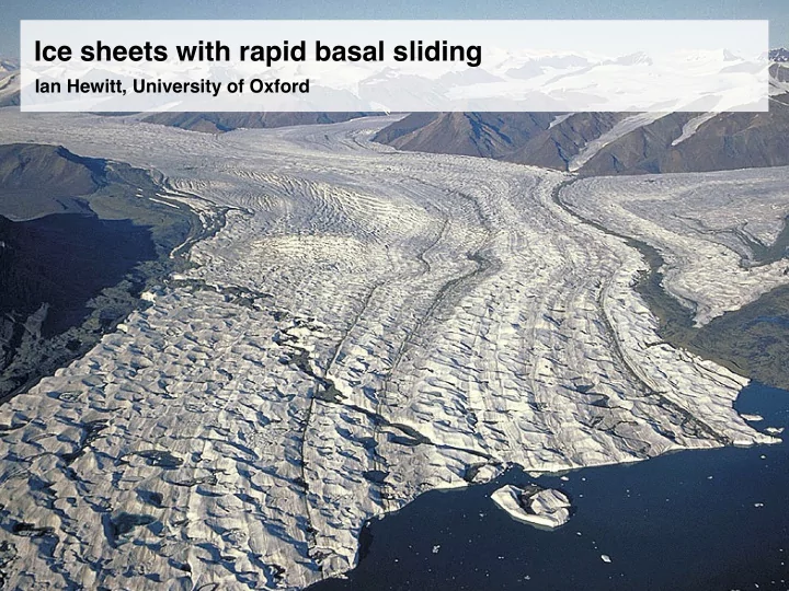
Ice sheets with rapid basal sliding
Ian Hewitt, University of Oxford
SLIDE 2 Antarctic ice sheet
Mouginot et al 2014 Marine Ice Sheet Collapse Potentially Under Way for the Thwaites Glacier Basin, West Antarctica
Ian Joughin, Benjamin E. Smith, Brooke Medley
Collapse of the West Antarctic Ice Sheet after local destabilization of the Amundsen Basin
Johannes Feldmanna,b and Anders Levermanna,b,1
Ice near the margins has accelerated substantially over the last decade McMillan et al 2014
SLIDE 3 30°W 60°W 60°W 60°W 90°W 120°W 120°E 120°E 120°E 90°E 90°E 90°E 7 ° S 8 ° S 60°E 60°E 60°E 30°E 0°E 150°W 150°E 150°E 150°E 180°E
Ice velocity (m year–1)
1,000 100 10 <1.5
B B' C' C
Ocean Ice Land 4,000 2,000 (MSL) 0
Elevation (m) West Antarctica
B' B
Ronne Ice Shelf Ellsworth Mountains Bentley Subglacial Trench Ross Ice Shelf Vertical exaggeration x80
Antarctic ice sheet
Bed elevation Ice speed
SLIDE 4
Sea level
20 40 60 –120 –80 –40 RSL (m) 50 100 150 200 250 300 350 400 450 500 dRSL (m kyr–1)
Grant et al 2014
Red Sea Relative Sea Level The glacial period is punctuated by several periods of rapid sea level rise (~1m/century) Time
SLIDE 5
The Greenland and Antarctic ice sheets contain ice equivalent to around 65m sea level Observations show rapid changes in ice dynamics can occur What mechanisms cause massive ice loss, and how rapid?
SLIDE 6
Basal sediments
This talk: Explore the dynamics of an ice sheet with a perfectly plastic bed Laboratory experiments on till samples suggest very weak dependence of stress on strain rate Shear strength depends on effective pressure (i.e. on pore pressure) τ0 = c + pe tan φ Iverson 2010 Most fast-moving ice is thought to be underlain by water-saturated sediments
SLIDE 7
Extreme Ice Survey - Time-lapse camera Khumbu glacier, Nepal
Glacier flow
~10,000,000 x real time
SLIDE 8 A simple ice-sheet model
∂h ∂t + ∂q ∂x = a Z ∂t ∂x q(x, t) = hu = Z s
b
u dz
Ice Bedrock
x z
z = s(x, t) h = s − b z = b(x) b u(x, z, t) ( Mass conservation Ice flux Force balance and boundary conditions (Stokes flow) b u(x, z, t) ( Net accumulation - melting (climate forcing) + a
SLIDE 9 Sliding at the bed
The fastest motion occurs as a plug flow u(x, z, t) ≈ u(x, t) Two mechanisms for sliding -
- a thin film of water between ice and bedrock
- lubrication by a layer of underlying water-saturated sediments (viscous)
z = b z = s
τb = ηs ds u τb ≈ −ρigh∂s ∂x | | τb = Cu From force balance ∂h ∂t = ∂ ∂x ✓ h2∂h ∂x ◆ + a Combining with mass conservation gives a diffusion equation for ice thickness Nye 1969
SLIDE 10
Plastic bed model
τb ≤ τ0 u = 0 τb = τ0 u ≥ 0 ( Consider the friction law Assuming deformation occurs, force balance becomes an equation for ice thickness So ice thickness is (almost) determined without reference to mass conservation or velocity ∂h ∂x = ∂b ∂x + τ0 ρigh Ice volume Global mass conservation − ∂x ≤ ρig h = 0 at x = xm ˙ V = Z xm a dx V = Z xm h dx
SLIDE 11 Example
a = λ(x0 − x) ( h = p 2h0(xm − x)1/2 p 2h0x1/2
m
˙ xm = λ ✓ x0 − 1 2xm ◆ xm
Accumulation, a Distance, x Elevation, z
ere xm = 2x0 Stable steady state ere xm = 2x0 Position-dependent accumulation h0 = τ0 ρig Global mass conservation ‘accumulation = ablation’
SLIDE 12 Distance, x Elevation, z
Ice sheet shrinks to nothing, or fills continental shelf a = λ(s − s0) ( − p 2h0x1/2
m
˙ xm = λ ✓2 3 p 2h0 x3/2
m − s0xm
◆ xm = 9 8 s2 h0 Elevation-dependent accumulation Eg.
Example
Unstable steady state h = p 2h0(xm − x)1/2 h0 = τ0 ρig Global mass conservation
SLIDE 13
Extreme Ice Survey - Time-lapse camera Columbia Glacier, Alaska
Marine-terminating glaciers
SLIDE 14 Marine-terminating glaciers
− = hf(x) = −ρo ρi b(x) Flotation thickness xm h − z = 0 z = b + hf
x z
z = b(x) − z = 0 xm qc
Mass conservation calving rate (includes
qm hm ˙ xm = qc h(x, t) =
SLIDE 15 Approximate force balance
0 = −∂p ∂x + ∂τxx ∂x + ∂τxz ∂z −∂x ∂x ∂z 0 = −∂p ∂z + ∂τxz ∂x + ∂τzz ∂z − ρig p − τzz = ρig(s − z) ( [h] [x] ∼ 10−3 Full force balance Small aspect ratio vertical balance approximately hydrostatic depth integrate horizontal balance, with τ xx ≈ 2ηi ∂u ∂x Note also, depth-integrated horizontal stress ∂ ∂x ✓ 4ηih∂u ∂x ◆ τb ρigh∂s ∂x = 0 ✓ ◆ Z s
b
−p + τxx dx = −1 2ρigh2 + 4ηih∂u ∂x
SLIDE 16
Continuity of longitudinal stress at the margin
Conditions at the marine margin
✓ ◆ −1 2ρigh2 + 4ηih∂u ∂x = −1 2ρogb2 at x = xm ρ calving rate (includes ocean-driven melting) Some models for calving prescribe a ‘rate’ Others prescribe an equilibrium-like ‘criteria’ - e.g. flotation condition h = hf ≡ −ρo ρi b xm qm = qc Z qc = qm − h ˙ xm
SLIDE 17 Full model
ε ∂ ∂x ✓ 4h∂u ∂x ◆ − τ∗ − h∂(b + h) ∂x = 0 ◆ ∂h ∂t + ∂q ∂x = a h = hf ε = ηi[a] [τ][x] ⌧ 1 ( r = ρo ρi ⇡ 1.1 (
x z
z = b(x) xm h(x, t) = q = 0 at x = 0 ε4h∂u ∂x = 1 2(h2 − h2
f/r)
at x = xm(t) (
τ∗ = 1 Boundary conditions flotation condition Non-dimensional equations
SLIDE 18 Numerical solutions
Distance, x
0.5 1 1.5 2
Elevation, z
2
Velocity, u
4
Distance, x
0.5 1 1.5 2
Elevation, z
2
Velocity, u
4
Distance, x
0.5 1 1.5 2
Elevation, z
2
Velocity, u
4
Steady states for constant accumulation a = 0.1 a = 1 a = 2
SLIDE 19 Margin boundary layer
h = ε1/4H u = ε−1/4U xm(t) x = ε1/2X ∂ ∂X (HU) = 0 ∂ ∂X ✓ 4H ∂U ∂X ◆ τ∗ + H ∂H ∂X = 0 Hf = ε−1/4rb(xm) ( UX = V
4Q + Q 4U 2V V 2 U U ! 0 V ! 0 as X ! 1
U V
( Q
Hf , 1−1/r 8
)
Longitudinal stress most important near margin rescale U = Q Hf V = 1 8(1 1/r)Hf at X = 0 Equations become Boundary / matching conditions HU = Q Only one value of allows the required trajectory Q Q = Qm(Hf) ⇡ (1 1/r) 8τ∗ H4
f
SLIDE 20 Reduced model
Away from the margin, ignore longitudinal stress τ∗ h∂h ∂x = 0 ∂h ∂t + ∂q ∂x = a h = 0 at x = xm at b(x) = O(ε1/4), hf = ε1/4Hf h = √ 2τ∗(xm − x)1/2 √ 2τ∗x1/2
m ˙
xm = Z xm a dx − Qm(Hf(xm)) Integrating mass conservation Distance, x
0.5 1 1.5 2
Flux, q
0.5 1 1.5 2
Z x a dx Qm(Hf(x)) Multiple steady states depending on bed slope (analogous to grounding lines, Schoof 2007)
SLIDE 21 More about calving
The boundary layer analysis can be generalised to find The role of calving in this model was to evacuate ice delivered to the margin If the processes responsible for calving cannot keep up, a floating ice shelf will form But if calving is more efficient, it may result in margin thickness above flotation hm ˙ xm = Qm(hm, hf) qc Replace flotation condition with
xm = qm qc qm = Qm(hm, hf) (
m
Qm
m f
SLIDE 22 Reduced model II
Away from the margin, ignore longitudinal stress τ∗ h∂h ∂x = 0 ∂h ∂t + ∂q ∂x = a h = 0 at x = xm at b(x) = O(ε1/4), hf = ε1/4Hf h = √ 2τ∗(xm − x)1/2 Integrating mass conservation √ 2τ∗x1/2
m ˙
xm = Z xm a dx − qc Z Qm(Hm, Hf) = qc Height above flotation adjusts to balance calving rate (Hindmarsh 2012)
SLIDE 23 Could meltwater-induced ice-sheet slow-down be a greater problem than acceleration?
For outlet glaciers, ‘accumulation’ includes inflow of ice from catchment basin - slow-down of surrounding ice will reduce ice supply, with potential rapid retreat. Changes in accumulation are the primary driver of the marine ice-sheet instability in this model. Recent observations suggest surface meltwater penetrating to the bed may slightly reduce, rather than increase, ice velocities.
Zwally et al 2002
1 2 3 4
Melt (w.e. m yr−1)
a
1985 1990 1995 2000
Year
2005 2010 2015 40 50 60 70 80 90 100 110 120
Velocity (m yr−1)
–0.1 m yr−2, P = 0.80 –1.5 m yr−2, P < 0.01 R2 = 0.79
b
400 600 800 1,000
Elevation (m.a.s.l.)
1,000 2,000
N
c
40 80 120
Area (km2)
Tedstone et al 2015
SLIDE 24
Summary
Ice-sheet beds can be modelled using plastic rheology (though should more realistically couple with water pressure) - enables simple studies of stability. Marine-terminating glaciers have potential for rapid retreat - slow-down of ice in the feeding catchment basin may initiate retreat. Calving processes act to keep the glacier tongue near flotation - but small differences in depth have large effect on ice flux.