
SLIDE 1
ST 370 Probability and Statistics for Engineers
Hypothesis Tests
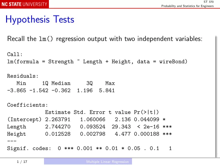
Recall the lm() regression output with two independent variables:
Call: lm(formula = Strength ~ Length + Height, data = wireBond) Residuals: Min 1Q Median 3Q Max
- 3.865 -1.542 -0.362
1.196 5.841 Coefficients: Estimate Std. Error t value Pr(>|t|) (Intercept) 2.263791 1.060066 2.136 0.044099 * Length 2.744270 0.093524 29.343 < 2e-16 *** Height 0.012528 0.002798 4.477 0.000188 ***
- Signif. codes:
0 *** 0.001 ** 0.01 * 0.05 . 0.1 1
1 / 17 Multiple Linear Regression