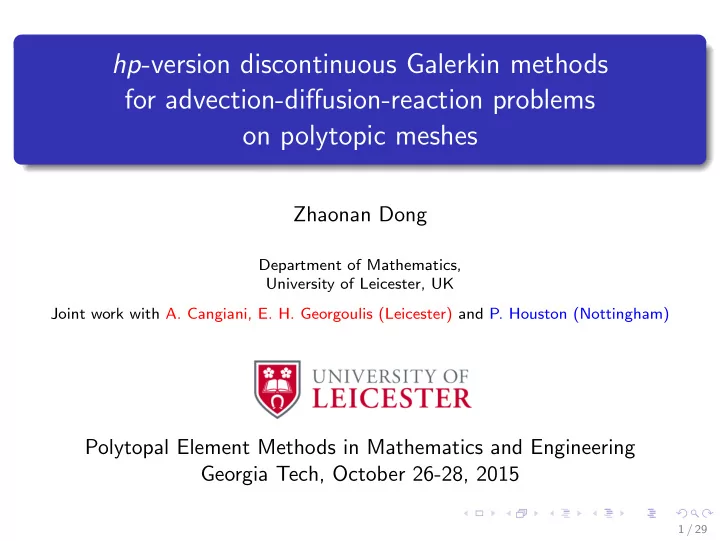
hp version discontinuous galerkin methods for advection
play

hp -version discontinuous Galerkin methods for - PowerPoint PPT Presentation

hp -version discontinuous Galerkin methods for advection-diffusion-reaction problems on polytopic meshes Zhaonan Dong Department of Mathematics, University of Leicester, UK Joint work with A. Cangiani, E. H. Georgoulis (Leicester) and P.


  1. hp -version discontinuous Galerkin methods for advection-diffusion-reaction problems on polytopic meshes Zhaonan Dong Department of Mathematics, University of Leicester, UK Joint work with A. Cangiani, E. H. Georgoulis (Leicester) and P. Houston (Nottingham) Polytopal Element Methods in Mathematics and Engineering Georgia Tech, October 26-28, 2015 1 / 29

  2. Model Problem Let Ω be a bounded open polyhedral domain in R d , d = 2 , 3. Consider the problem d d � � L u ≡ − ∂ j ( a ij ( x ) ∂ i u ) + b i ( x ) ∂ i u + c ( x ) u = f ( x ) , (1) i , j =1 i =1 where c ∈ L ∞ (Ω), f ∈ L 2 (Ω), and b := ( b 1 , b 2 , . . . , b d ) ⊤ ∈ [ W 1 ∞ (Ω)] d . i , j =1 such that a ij ∈ L ∞ (¯ a = { a ij } d Ω), with ξ ⊤ a ( x ) ξ ≥ 0 x ∈ ¯ ∀ ξ ∈ R d , a.e Ω . (2) 2 / 29

  3. Model Problem Let Ω be a bounded open polyhedral domain in R d , d = 2 , 3. Consider the problem d d � � L u ≡ − ∂ j ( a ij ( x ) ∂ i u ) + b i ( x ) ∂ i u + c ( x ) u = f ( x ) , (1) i , j =1 i =1 where c ∈ L ∞ (Ω), f ∈ L 2 (Ω), and b := ( b 1 , b 2 , . . . , b d ) ⊤ ∈ [ W 1 ∞ (Ω)] d . i , j =1 such that a ij ∈ L ∞ (¯ a = { a ij } d Ω), with ξ ⊤ a ( x ) ξ ≥ 0 x ∈ ¯ ∀ ξ ∈ R d , a.e Ω . (2) Under hypothesis (2), (1) is termed a partial differential equation with non-negative characteristic form. This class includes elliptic, parabolic, hyperbolic, mixed-type PDEs. 2 / 29

  4. Model Problem Let Γ signify the union of its ( d − 1)-dimensional open faces of ∂ Ω. Γ + n ⊤ a ( x ) n = 0 Γ N Γ − Ω n ⊤ a ( x ) n > 0 Γ D b Γ D Problem (1) is well-posed under (standard) hypothesis: c 0 ( x ) 2 := c ( x ) − 1 2 ∇ · b ( x ) ≥ γ 0 > 0 a.e x ∈ Ω . (3) 3 / 29

  5. Model Problem Let Γ signify the union of its ( d − 1)-dimensional open faces of ∂ Ω. Γ + n ⊤ a ( x ) n = 0 Γ N Γ − Ω n ⊤ a ( x ) n > 0 Γ D b Γ D Problem (1) is well-posed under (standard) hypothesis: c 0 ( x ) 2 := c ( x ) − 1 2 ∇ · b ( x ) ≥ γ 0 > 0 a.e x ∈ Ω . (3) Aim: Derive and analyse hp -version dG methods on extremely general polytopic meshes for this problem. 3 / 29

  6. Challenges and their resolution Classical hp -inverse estimates not sharp for polytopic elements with arbitrarily small ( d − k )-dim faces, k = 1 , . . . , d − 1. Inverse estimates dictate IPDG penalisation constant. 4 / 29

  7. Challenges and their resolution Classical hp -inverse estimates not sharp for polytopic elements with arbitrarily small ( d − k )-dim faces, k = 1 , . . . , d − 1. Inverse estimates dictate IPDG penalisation constant. → new sharp hp -inverse estimates for polytopic elements with arbitrarily small ( d − k )-dim faces 4 / 29

  8. Challenges and their resolution Classical hp -inverse estimates not sharp for polytopic elements with arbitrarily small ( d − k )-dim faces, k = 1 , . . . , d − 1. Inverse estimates dictate IPDG penalisation constant. → new sharp hp -inverse estimates for polytopic elements with arbitrarily small ( d − k )-dim faces No sharp hp -approximation results for L 2 -projector over polytopic meshes. L 2 -projector key for first order terms Houston, Schwab & S¨ uli (’02) . 4 / 29

  9. Challenges and their resolution Classical hp -inverse estimates not sharp for polytopic elements with arbitrarily small ( d − k )-dim faces, k = 1 , . . . , d − 1. Inverse estimates dictate IPDG penalisation constant. → new sharp hp -inverse estimates for polytopic elements with arbitrarily small ( d − k )-dim faces No sharp hp -approximation results for L 2 -projector over polytopic meshes. L 2 -projector key for first order terms Houston, Schwab & S¨ uli (’02) . → error analysis via hp -inf-sup stability on stronger norms. ` a la Johnson & Pitk¨ aranta (’86), Buffa, Hughes & Sangalli (’06), Ayuso & Marini (’09),... 4 / 29

  10. The Finite Element Space for DGFEMs DGFEMs are not restricted to employing standard polynomial spaces mapped from a reference frame. In this work, the FE space are constructed with following properties: Polynomial basis are defined over physical meshes On each element κ , we employ the total degree space P p ( κ ). 5 / 29

  11. The Finite Element Space for DGFEMs DGFEMs are not restricted to employing standard polynomial spaces mapped from a reference frame. In this work, the FE space are constructed with following properties: Polynomial basis are defined over physical meshes On each element κ , we employ the total degree space P p ( κ ). Definition of Finite Element Space: mesh T : disjoint subdivision of Ω into polygons/polyhedra; discretisation parameters : ◮ mesh size h κ := diam ( κ ), κ ∈ T ; ◮ polynomial degree vector p : ( p κ ∈ N , κ ∈ T ) The DG finite element space S p T with respect to T and p defined by: S p T := { u ∈ L 2 (Ω) : u | κ ∈ P p κ ( κ ) , κ ∈ T } , 5 / 29

  12. Notation for DGFEMs Average { {·} } of v and q at x ∈ F : � 1 � 1 2 ( v i + v j ) , F ⊂ Γ int 2 ( q i + q j ) , F ⊂ Γ int { { v } } := , { { q } } := . v i , F ⊂ Γ q i , F ⊂ Γ Jump of v and q at x ∈ F : � v i n i + v j n j , � q i · n i + q j · n j , F ⊂ Γ int F ⊂ Γ int [ [ v ] ] := , [ [ q ] ] := . v i n i , F ⊂ Γ q i · n i , F ⊂ Γ Upwind jump of (scalar-valued) function v across a face F : � v + κ − v − κ , F ⊂ ∂ − κ \ Γ ⌊ v ⌋ := v + κ , F ⊂ Γ v + κ and v − κ upwind and downwind w.r.t b values. 6 / 29

  13. Weak formulation of DGFEM For simplicity of presentation, we assume a ∈ [ S 0 T ] d × d sym . and that b · ∇ ξ ∈ S p T , for ξ ∈ S p T . (important for p -version bounds.) 7 / 29

  14. Weak formulation of DGFEM For simplicity of presentation, we assume a ∈ [ S 0 T ] d × d sym . and that b · ∇ ξ ∈ S p T , for ξ ∈ S p T . (important for p -version bounds.) Then the IP DGFEM is given by: find u h ∈ S p T such that B ( u h , v h ) = ℓ ( v h ) , (4) for all v h ∈ S p T . Here, the bilinear form B ( · , · ) : S p T × S p T → R is defined as the sum of two parts B ( u , v ) := B ar ( u , v ) + B d ( u , v ) , 7 / 29

  15. Weak formulation of DGFEM The first part B ar accounts for the advection and reaction terms: � � � � B ar ( u , v ) := b · ∇ u + cu v d x κ κ ∈T � � ( b · n ) ⌊ u ⌋ v + d s − ( b · n ) u + v + d s , � � − ∂ − κ \ Γ ∂ − κ ∩ (Γ D ∪ Γ − ) κ ∈T κ ∈T and the second part B d is responsible for the diffusion term: � � � B d ( u , v ) := a ∇ u · ∇ v d x + σ [ [ u ] ] · [ [ v ] ] d s κ Γ int ∪ Γ D κ ∈T � � � − { { a ∇ h u } } · [ [ v ] ] + { { a ∇ h v } } · [ [ u ] ] d s . Γ int ∪ Γ D 8 / 29

  16. Weak formulation of DGFEM The linear functional ℓ : S p T → R is defined by � � ( b · n ) g D v + d s � � ℓ ( v ) := fv d x − κ ∂ − κ ∩ (Γ D ∪ Γ − ) κ ∈T κ ∈T � � � � − g D ( a ∇ h v ) · n − σ v d s + g N v d s . Γ D Γ N Remark: The discontinuity-penalization parameter σ ∈ L ∞ (Γ int ∪ Γ D ) will be defined later. 9 / 29

  17. hp -inverse estimate from trace For v ∈ P p ( κ ), a classical inverse estimate on the simplex κ F ♭ gives: L 2 ( F ) � p 2 | F | ♭ ) � p 2 | F | � v � 2 ♭ | � v � 2 ♭ | � v � 2 L 2 ( κ ) . L 2 ( κ F | κ F | κ F Note: This is not sharp when | F | → 0 ! κ F ♭ F 10 / 29

  18. hp -inverse estimate from trace For v ∈ P p ( κ ), a classical inverse estimate on the simplex κ F ♭ gives: L 2 ( F ) � p 2 | F | ♭ ) � p 2 | F | � v � 2 ♭ | � v � 2 ♭ | � v � 2 L 2 ( κ ) . L 2 ( κ F | κ F | κ F Note: This is not sharp when | F | → 0 ! κ F Using some developments ♭ from Georgoulis (’2008) , we can F show the following inverse estimate which remains sharp when | F | → 0: 10 / 29

  19. Inverse estimate lemma Lemma (Trace-inverse estimate) If κ ∈ ˜ T then for each v ∈ P p ( κ ) , we have the inverse estimate L 2 ( F ) ≤ C INV ( p , κ, F ) p 2 | F | � v � 2 | κ | � v � 2 L 2 ( κ ) , (5) � � with  | κ | if κ ∈ ˜ ♭ | , p 2 d  min , T ,   ♭ ⊂ κ | κ F sup κ F  C INV ( p , κ, F ) := C inv | κ | if κ ∈ T \ ˜  ♭ | , T ,   ♭ ⊂ κ | κ F sup κ F  11 / 29

  20. Inverse estimate lemma Lemma (Trace-inverse estimate) If κ ∈ ˜ T then for each v ∈ P p ( κ ) , we have the inverse estimate L 2 ( F ) ≤ C INV ( p , κ, F ) p 2 | F | � v � 2 | κ | � v � 2 L 2 ( κ ) , (5) � � with  | κ | if κ ∈ ˜ ♭ | , p 2 d  min , T ,   ♭ ⊂ κ | κ F sup κ F  C INV ( p , κ, F ) := C inv | κ | if κ ∈ T \ ˜  ♭ | , T ,   ♭ ⊂ κ | κ F sup κ F  Lemma ( H 1 -inverse estimate) If for each v ∈ P p ( κ ) , we have the inverse estimate p 4 L 2 ( κ ) ≤ ˜ �∇ v � 2 � v � 2 C inv L 2 ( κ ) , (6) h 2 κ where the constant ˜ C inv is independent of discretization parameter h κ , p κ . 11 / 29

  21. Main Result Let penalisation σ : Γ \ Γ N → R + be defined facewise by  a κ p 2 C INV ( p κ , κ, F ) ¯ κ | F | � � C σ max , x ∈ F ⊂ Γ int , F = ∂κ 1 ∩ ∂κ 2 ,    | κ | κ ∈{ κ 1 ,κ 2 } σ ( x ) := a κ p 2 | F | C σ C INV ( p κ , κ, F ) ¯ , x ∈ F ⊂ Γ D , F = ∂κ ∩ Γ D ,    | κ | (7) with C σ > 0 large enough, and independent of p , | F | , and | κ | . 12 / 29

Download Presentation
Download Policy: The content available on the website is offered to you 'AS IS' for your personal information and use only. It cannot be commercialized, licensed, or distributed on other websites without prior consent from the author. To download a presentation, simply click this link. If you encounter any difficulties during the download process, it's possible that the publisher has removed the file from their server.

Recommend


More recommend