Homographies and Estimating Extrinsics Instructor - Simon Lucey - PowerPoint PPT Presentation
Homographies and Estimating Extrinsics Instructor - Simon Lucey 16-423 - Designing Computer Vision Apps Review: Motivation Adapted from: Computer vision: models, learning and inference. Simon J.D. Prince Review: Pinhole Camera Instead model
Homographies and Estimating Extrinsics Instructor - Simon Lucey 16-423 - Designing Computer Vision Apps
Review: Motivation Adapted from: Computer vision: models, learning and inference. Simon J.D. Prince
Review: Pinhole Camera Instead model impossible but more convenient Real camera image virtual image is inverted Adapted from: Computer vision: models, learning and inference. Simon J.D. Prince
Today • Fitting Warp Functions. • Estimating Intrinsics.
Euclidean warp • Consider viewing a fronto-parallel plane at a fixed distance D. • In homogeneous coordinates, the imaging equations are: Plane at Point is on 3D rotation matrix known plane becomes 2D (in plane) ( w =0) distance D Adapted from: Computer vision: models, learning and inference. Simon J.D. Prince
Euclidean warp • Simplifying • Rearranging the last equation Adapted from: Computer vision: models, learning and inference. Simon J.D. Prince
Euclidean warp Homogeneous: Cartesian: For short: Adapted from: Computer vision: models, learning and inference. Simon J.D. Prince
Euclidean warp Homogeneous: Cartesian: For short: How many unknowns? Adapted from: Computer vision: models, learning and inference. Simon J.D. Prince
Estimating the Euclidean Warp N ˆ X Ω , ˆ τ = arg min η { x n − euc[ w n , Ω , τ ] } Ω , τ n =1
Estimating the Euclidean Warp N ˆ X || x n − euc[ w n , Ω , τ ] || 2 Ω , ˆ τ = arg min 2 Ω , τ n =1
Estimating the Euclidean Warp N ˆ X || x n − euc[ w n , Ω , τ ] || 2 Ω , ˆ τ = arg min 2 Ω , τ n =1 N X || x n − Ω w n + τ || 2 = arg min 2 Ω , τ n =1
Estimating the Euclidean Warp N ˆ X || x n − euc[ w n , Ω , τ ] || 2 Ω , ˆ τ = arg min 2 Ω , τ n =1 N X || x n − Ω w n + τ || 2 = arg min 2 Ω , τ n =1 s.t. Ω T Ω = I , det( Ω ) = 1
Reminder: Non-Convex Set 9
Reminder: Non-Convex Set 9
Reminder: Non-Convex Set 9
Estimating the Euclidean Warp N ˆ X || ( x n − µ x ) − Ω ( w n − µ w ) || 2 Ω = arg min 2 Ω n =1 s.t. Ω T Ω = I , det( Ω ) = 1 N N µ x = 1 µ w = 1 X X x n , w n N N n =1 n =1
Estimating the Euclidean Warp • In MATLAB this becomes, >> [U,S,V] = svd(B*A’,0); >> Omega = U*V’; • SVD method works for ONLY very specific objectives. • Extremely useful as it allows us to find closed form solutions to a non-convex problem ( very rare ).
Similarity warp • Consider viewing fronto-parallel plane at unknown distance D • By same logic as before we have Adapted from: Computer vision: models, learning and inference. Simon J.D. Prince
Similarity warp • Simplifying: • Multiply each equation by : Adapted from: Computer vision: models, learning and inference. Simon J.D. Prince
Similarity warp • Simplifying: • Incorporate the constants by defining: Adapted from: Computer vision: models, learning and inference. Simon J.D. Prince
Similarity warp Homogeneous: Cartesian: For short:
Similarity warp Homogeneous: Cartesian: For short: How many unknowns?
Estimating the Similarity Warp • Simplifying: • Since,
Estimating the Similarity Warp • Rearranging: • Form system of equations:
Estimating the Similarity Warp • In MATLAB this becomes, >> p = A\x; • Since p stems form a convex set, simply use “backslash”!!!
Estimating the Similarity Warp • In MATLAB this becomes, >> p = A\x; • Since p stems form a convex set, simply use “backslash”!!!
Estimating the Similarity Warp • In MATLAB this becomes, >> p = A\x; • Since p stems form a convex set, simply use “backslash”!!!
Affine warp When variation in depth is comparable to Affine transform describes mapping distance to object then the affine well when the depth variation within the transformation is not a good model. planar object is small and the camera Here we need the homography. is far away. Adapted from: Computer vision: models, learning and inference. Simon J.D. Prince
Affine warp Homogeneous: Cartesian: For short:
Affine warp Homogeneous: Cartesian: For short: How many unknowns?
Estimating the Affine Warp • Rearranging: • Form system of equations: • In MATLAB this becomes, >> p = A\x;
Homography • Start with basic projection equation: • Combining these two matrices we get: Adapted from: Computer vision: models, learning and inference. Simon J.D. Prince
Homography Homogeneous: Cartesian: For short:
Homography Homogeneous: Cartesian: For short: How many unknowns?
Homography Estimation • Re-arrange cartesian equations, • Form linear system φ 11 0 0 0 − 1 − u 1 − v 1 y 1 u 1 y 1 v 1 y 1 φ 12 1 0 0 0 u 1 v 1 − x 1 u 1 − x 1 v 1 − x 1 φ 13 0 0 0 − 1 − u 2 − v 2 y 2 u 2 y 2 v 2 y 2 φ 21 1 0 0 0 u 2 v 2 − x 2 u 2 − x 2 v 2 − x 2 = 0 , φ 22 . . . . . . . . . . . . . . . . . . φ 23 . . . . . . . . . φ 31 0 0 0 − 1 − u I − v I y I u I y I v I y I φ 32 1 0 0 0 u I v I − x I u I − x I v I − x I φ 33 Adapted from: Computer vision: models, learning and inference. Simon J.D. Prince
Homography Estimation • In MATLAB this becomes, >> [U,S,V] = svd(A); >> Phi = reshape(V(:,end),[3,3])’; • Both sides are 3x1 vectors; should be parallel, so cross product will be zero • For you to try MATLAB, >> x = [randn(2,1);1]; cross(x,4*x)
Caution… • Approach only minimizes algebraic error NOT the re- projection error!!! • Need to employ non-linear optimization.
Today • Fitting Warp Functions. • Estimating Extrinsics.
Estimating Extrinsics
Estimating Extrinsics • Writing out the camera equations in full • Estimate the homography from matched points • Factor out the intrinsic parameters Adapted from: Computer vision: models, learning and inference. Simon J.D. Prince
Estimating Extrinsics • Find the last column using the cross product of first two columns • Make sure the determinant is 1. If it is -1, then multiply last column by -1. • Find translation scaling factor between old and new values • Finally, set Adapted from: Computer vision: models, learning and inference. Simon J.D. Prince
Augmented Reality
Transformations between images • So far we have considered transformations between the image and a plane in the world • Now consider two cameras viewing the same plane • There is a homography between camera 1 and the plane and a second homography between camera 2 and the plane • It follows that the relation between the two images is also a homography
Camera under pure rotation Special case is camera under pure rotation. Homography can be showed to be
Camera under pure rotation Special case is camera under pure rotation. Homography can be showed to be Why is this?
Panorama Example a) b) c) d)
More to read… • Prince et al. • Chapter 14, Sections 1-4. • Chapter 15, Sections 1-6.
Recommend
More recommend
Explore More Topics
Stay informed with curated content and fresh updates.
