
SLIDE 1
Homogeneous transforms
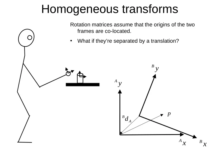
Rotation matrices assume that the origins of the two frames are co-located.
- What if they’re separated by a translation?
x
A
p
y
A
A Bd
y
B
x
B
Homogeneous transforms Rotation matrices assume that the origins of - - PowerPoint PPT Presentation
Homogeneous transforms Rotation matrices assume that the origins of the two frames are co-located. What if theyre separated by a translation? B y A y p B d A A x B x Homogeneous transform B y A y (same point, two
Rotation matrices assume that the origins of the two frames are co-located.
A
A
A Bd
B
B
A ˆ
A ˆ
B Ad
B ˆ
B ˆ
B A B B A A
B
A
A
p
A
b ad
B
B
B B A B A
33 32 31 23 22 21 13 12 11
B B A B z A y A x A
B A B B A A
A BT
A
A
B
B
A
B
A BT
x
A
y
A
x
B
y
B
l θ z
A
z
B
B AR
B
x
A
y
A
z z B
A ,
x
B
y
B
θ
A B A B A B
B
What’s ?
b aT
a
a
a
b
b
b
4 4 π π
a
This arm rotates about the axis. a
x
A ˆ
y
A ˆ
z
A ˆ
x
c ˆ
y
c ˆ
z
c ˆ
θ φ l
θ φ θ φ θ φ φ θ θ φ φ θ φ φ φ φ θ θ θ θ
c b b a c a
φ θ θ φ θ φ θ φ φ φ φ θ θ θ φ φ θ
a c a c a
x
A ˆ
y
A ˆ
z
A ˆ
x
c ˆ
y
c ˆ
z
c ˆ
θ φ l
c
φ θ φ φ θ θ φ θ φ θ φ φ θ θ φ φ θ
c c a a
−
1 A B T A B T A B A B
A B A A B B
A B B T A B A
Can also derive it from the forward Homogeneous transform:
−
1
B A B A
where
A ˆ
A ˆ
B Ad
B ˆ
B ˆ
B A A A B B A A B A A B B
B
A
B AT
A
A
B
B
A
B
B
− = 1 ) cos( ) sin( ) sin( ) cos( θ θ θ θ
B AR
− = l d A
B
−
1
B A A B
−
1 A B T A B T A B A B
= − − = − ) sin( ) cos( 1 ) cos( ) sin( ) sin( ) cos( θ θ θ θ θ θ l l l d R
A B B A
What’s ?
a bT
a
a
a
b
b
b
4 4 π π
a
+ + + +
4 4 4 4 π π π π
θ θ θ θ θ θ θ θ
b
3 2 2 1 1 3
1
2
3
1
1
2
2
3
3
1
l
2
l
3
l
Base to eff transform Transform associated w/ link 1 Transform associated w/ link 2 Transform associated w/ link 3
3 2 2 1 1 3
1 1 1 1 1 1 1 1 1
2 2 2 2 2 2 2 2 2 1
1
2
3
1
1
2
2
3
3
1
l
2
l
3
l
3 2 2 1 1 3
3 3 3 3 3 3 3 3 3 2
1
2
3
1
1
2
2
3
3
1
l
2
l
3
l
3 2 2 1 1 3
3 3 3 3 3 3 3 3 2 2 2 2 2 2 2 2 1 1 1 1 1 1 1 1 3
123 3 12 2 1 1 123 123 123 3 12 2 1 1 123 123 3
can encode the kinematics of a manipulator
approach: DH (Denavit-Hartenberg) parameters.
for arbitrary mechanisms. x y
1
q
z
2
q
3
q
x
1
y
1
y
2
x
2
x
3
y
3
1
l
2
l
3
l
x z
1
q
y
2
q
3
q
x
1
z
1
z
2
x
2
x
3
z
3
1
l
2
l
3
l
i i i i
i i i i i i i i
i i α α α α θ θ θ θ
Then, translate by along x axis
i
and rotate by about x axis
i
First, translate by along z axis
i
and rotate by about z axis
i
i i i i i i i i
i i α α α α θ θ θ θ
i i i
i i i i i i i i i i i i i i
α α θ α θ α θ θ θ α θ α θ θ
1
1
θ
1
1
1
1
2
2
Then, translate by along x axis
i
and rotate by about x axis
i
First, translate by along z axis
i
and rotate by about z axis
i
i i i i
( ) ( ) ( ) ( )
i i i i
a x trans x rot d z trans z rot
, , , , α θ
xform 1 2
i
i
i
i
1
1
1
1
2
2
2
2
1
q
2
q
3
q
1
1
2
2
3
3
1
l
2
l
3
l
i
i
i
i
1
1
2
2
1 2 3
3
3
x y
1
q
z
2
q
3
q
x
1
y
1
y
2
x
2
x
3
y
3
1
l
2
l
3
l
1 2 3
i
a
i
α
i
d
i
θ
1
l
1
q
2
l
2
q
3
l
3
q
− = 1 1
1 1 1 1 1 1
1 1 1 q q q q q q
s l c s c l s c T
− = 1 1
2 2 2 2 2 2
2 2 2 1 q q q q q q
s l c s c l s c T
− = 1 1
3 3 3 3 3 3
3 3 3 2 q q q q q q
s l c s c l s c T
3 2 2 1 1 3
1
q
2
q
3
q
x y z
1
z
1
x
2
z
2
x
2
y
3
z
3
y
3
x
1
l
2
l
3
l
1
q
2
q
3
q
x y z
1
z
1
x
2
z
2
x
2
y
3
z
3
y
3
x
1
l
2
l
3
l
i
i
i
i
1
2 π
1
2
2 2 π
1 2 3
3
3
1
q
1
1
l
2
q
3
q
4
q
1
1
2
2
2
2
2
2
1
q
1
1
l
2
q
3
q
4
q
1
1
2
2
2
2
2
2
1 2 3 4
i
a
i
α
i
d
i
θ
1
l
1
q
2
q
3
q
π
4
q
2
l
3
l
4
l