Hill Climbing Many search spaces are too big for systematic search. - - PowerPoint PPT Presentation

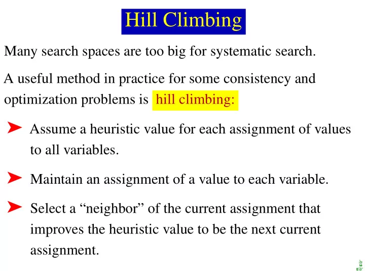
Hill Climbing

Many search spaces are too big for systematic search. A useful method in practice for some consistency and

• ptimization problems is hill climbing:

➤ Assume a heuristic value for each assignment of values

to all variables.

➤ Maintain an assignment of a value to each variable. ➤ Select a “neighbor” of the current assignment that

improves the heuristic value to be the next current assignment.

☞ ☞

Selecting Neighbors in Hill Climbing

➤ When the domains are small or unordered, the neighbors

• f a node correspond to choosing another value for one
• f the variables.

➤ When the domains are large and ordered, the neighbors of

a node are the adjacent values for one of the dimensions.

➤ If the domains are continuous, you can use

Gradient ascent: change each variable proportional to the gradient of the heuristic function in that direction. The value of variable Xi goes from vi to vi + η ∂h

∂Xi .

Gradient descent: go downhill; vi becomes vi − η ∂h

∂Xi .

☞ ☞ ☞

Problems with Hill Climbing

Foothills local maxima that are not global maxima Plateaus heuristic values are uninformative Ridge foothill where n-step lookahead might help Ignorance of the peak

Ridge Foothill Plateau

☞ ☞ ☞

Randomized Algorithms

➤ Consider two methods to find a maximum value: ➣ Hill climbing, starting from some position, keep

moving uphill & report maximum value found

➣ Pick values at random & report maximum value found ➤ Which do you expect to work better to find a maximum? ➤ Can a mix work better?

☞ ☞ ☞

Randomized Hill Climbing

As well as uphill steps we can allow for:

➤ Random steps: move to a random neighbor. ➤ Random restart: reassign random values to all variables.

Which is more expensive computationally?

☞ ☞ ☞

1-Dimensional Ordered Examples

Two 1-dimensional search spaces; step right or left:

➤ Which method would most easily find the maximum? ➤ What happens in hundreds or thousands of dimensions? ➤ What if different parts of the search space have different

structure?

☞ ☞ ☞

Stochastic Local Search for CSPs

➤ Goal is to find an assignment with zero unsatisfied

relations.

➤ Heuristic function: the number of unsatisfied relations. ➤ We want an assignment with minimum heuristic value. ➤ Stochastic local search is a mix of: ➣ Greedy descent: move to a lowest neighbor ➣ Random walk: taking some random steps ➣ Random restart: reassigning values to all variables

☞ ☞ ☞

Greedy Descent

➤ It may be too expensive to find the variable-value pair

that minimizes the heuristic function at every step.

➤ An alternative is: ➣ Select a variable that participates in the most number

• f conflicts.

➣ Choose a (different) value for that variable that

resolves the most conflicts. The alternative is easier to compute even if it doesn’t always maximally reduce the number of conflicts.

☞ ☞ ☞

Random Walk

You can add randomness:

➤ When choosing the best variable-value pair, randomly

sometimes choose a random variable-value pair.

➤ When selecting a variable then a value: ➣ Sometimes choose a random variable. ➣ Sometimes choose, at random, a variable that

participates in a conflict (a red node).

➣ Sometimes choose a random variable. ➤ Sometimes choose the best value and sometimes choose

a random value.

☞ ☞ ☞

Comparing Stochastic Algorithms

➤ How can you compare three algorithms when ➣ one solves the problem 30% of the time very quickly

but doesn’t halt for the other 70% of the cases

➣ one solves 60% of the cases reasonably quickly but

doesn’t solve the rest

➣ one solves the problem in 100% of the cases, but

slowly?

➤ Summary statistics, such as mean run time, median run

time, and mode run time don’t make much sense.

☞ ☞ ☞

Runtime Distribution

➤ Plots runtime (or number of steps) and the proportion (or

number) of the runs that are solved within that runtime.

0.1 0.2 0.3 0.4 0.5 0.6 0.7 0.8 0.9 1

1 10 100 1000

☞ ☞ ☞

Variant: Simulated Annealing

➤ Pick a variable at random and a new value at random. ➤ If it is an improvement, adopt it. ➤ If it isn’t an improvement, adopt it probabilistically

depending on a temperature parameter, T.

➣ With current node n and proposed node n′ we move to

n′ with probability e(h(n′)−h(n))/T

➤ Temperature can be reduced.

☞ ☞ ☞

Tabu lists

➤ To prevent cycling we can maintain a tabu list of the k

last nodes visited.

➤ Don’t allow a node that is already on the tabu list. ➤ If k = 1, we don’t allow a node to the same value. ➤ We can implement it more efficiently than as a list of

complete nodes.

➤ It can be expensive if k is large.

☞ ☞ ☞

Parallel Search

➤ Idea: maintain k nodes instead of one. ➤ At every stage, update each node. ➤ Whenever one node is a solution, it can be reported. ➤ Like k restarts, but uses k times the minimum number of

steps.

☞ ☞ ☞

Beam Search

➤ Like parallel search, with k nodes, but you choose the k

best out of all of the neighbors.

➤ When k = 1, it is hill climbing. ➤ When k = ∞, it is breadth-first search. ➤ The value of k lets us limit space and parallelism. ➤ Randomness can also be added.

☞ ☞ ☞

Stochastic Beam Search

➤ Like beam search, but you probabilistically choose the k

nodes at the next generation.

➤ The probability that a neighbor is chosen is proportional

to the heuristic value.

➤ This maintains diversity amongst the nodes. ➤ The heuristic value reflects the fitness of the node. ➤ Like asexual reproduction: each node gives its mutations

and the fittest ones survive.

☞ ☞ ☞

Genetic Algorithms

➤ Like stochastic beam search, but pairs are nodes are

combined to create the offspring:

➤ For each generation: ➣ Randomly choose pairs of nodes where the fittest

individuals are more likely to be chosen.

➣ For each pair, perform a cross-over: form two

• ffspring each taking different parts of their parents:

➣ Mutate some values ➤ Report best node found.

☞ ☞ ☞

Crossover

➤ Given two nodes:

X1 = a1, X2 = a2, . . . , Xm = am X1 = b1, X2 = b2, . . . , Xm = bm

➤ Select i at random. ➤ Form two offspring:

X1 = a1, . . . , Xi = ai, Xi+1 = bi+1, . . . , Xm = bm X1 = b1, . . . , Xi = bi, Xi+1 = ai+1, . . . , Xm = am

➤ Note that this depends on an ordering of the variables. ➤ Many variations are possible.

☞ ☞ ☞

Example: Crossword Puzzle

1 2 3 4

Words: ant, big, bus, car, has book, buys, hold, lane, year beast, ginger, search, symbol, syntax

☞ ☞