high velocity impact damage behavior of graphite epoxy
play

HIGH-VELOCITY IMPACT DAMAGE BEHAVIOR OF GRAPHITE-EPOXY COMPOSITE - PDF document

18 TH INTERNATIONAL CONFERENCE ON COMPOSITE MATERIALS HIGH-VELOCITY IMPACT DAMAGE BEHAVIOR OF GRAPHITE-EPOXY COMPOSITE LAMINATES K. Woo 1* , I. Kim 2 , S.C. Ha 2 , H. Shin 2 , and J.H. Kim 3 1 School of Civil Engineering, Chungbuk National


  1. 18 TH INTERNATIONAL CONFERENCE ON COMPOSITE MATERIALS HIGH-VELOCITY IMPACT DAMAGE BEHAVIOR OF GRAPHITE-EPOXY COMPOSITE LAMINATES K. Woo 1* , I. Kim 2 , S.C. Ha 2 , H. Shin 2 , and J.H. Kim 3 1 School of Civil Engineering, Chungbuk National University, Cheongju, Korea 2 Department of Aerospace Engineering, Chungnam National University, Daejeon, Korea 3 Agency for Defense Development, Daejeon, Korea * Corresponding author(kw3235@chungbuk.ac.kr) Keywords : high-velocity impact, composite laminates, impact damage, acoustic emission, failure analysis, penetration velocity, element erosion magnetic velocity sensors for measuring the steel 1 Introduction ball velocity, AE (acoustic emission) sensor and The high-velocity impact of small objects can cause supporting fixtures. The velocity limit of the air gun severe damage to the laminated composite structures is approximately 325 m/s. The two magnetic sensors (e.g., Refs. [1-3]). Proper understanding of high- are mounted at the end of gun barrel at a distance of velocity impact damage behavior is one of the key 10 cm apart and the other two magnetic sensors are elements for the establishment of structural integrity mounted at the rear of impact specimen for for aerospace structures, and thus, has been the focus measuring the residual velocity after penetration. of many researches over the past several decades (e.g, Refs. [4-5]). In this study, a series of high-velocity impact tests were performed to investigate the impact damage behavior of laminated composites. In the experiment, the air gun impact tester was used, and the ballistic and residual velocity was measured. Also, the acoustic emission of the laminate was recorded for further examination. In the analysis, a numerical simulation procedure was developed in which LS- DYNA finite element models were generated and analyzed. The simulation results were compared to 
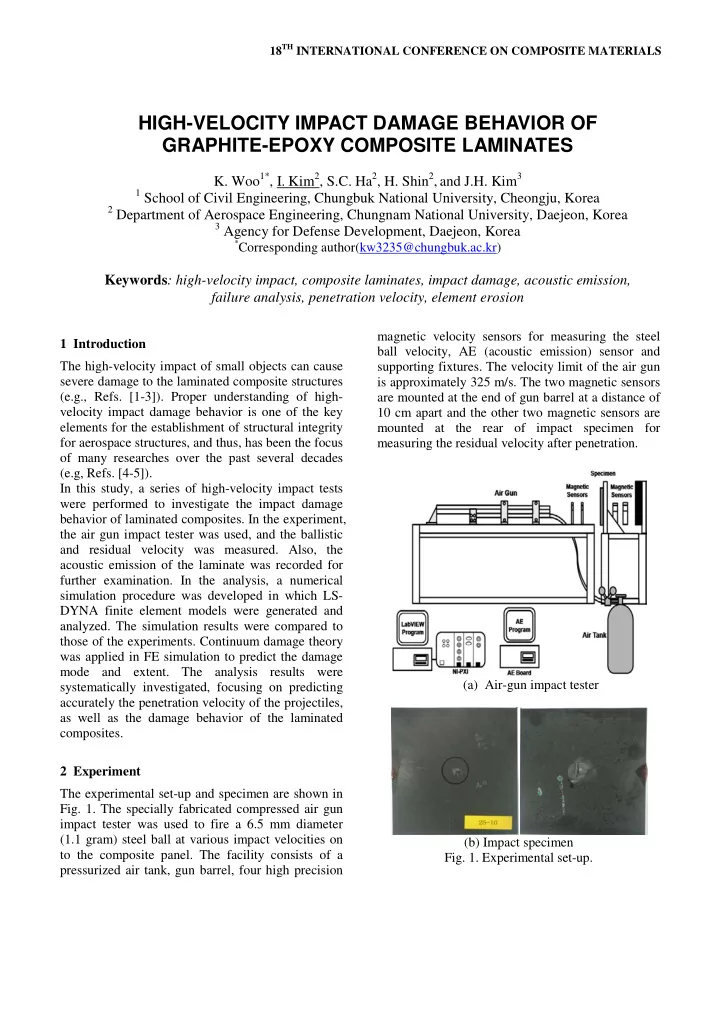
those of the experiments. Continuum damage theory was applied in FE simulation to predict the damage mode and extent. The analysis results were (a) Air-gun impact tester systematically investigated, focusing on predicting accurately the penetration velocity of the projectiles, as well as the damage behavior of the laminated composites. 2 Experiment The experimental set-up and specimen are shown in Fig. 1. The specially fabricated compressed air gun impact tester was used to fire a 6.5 mm diameter (1.1 gram) steel ball at various impact velocities on (b) Impact specimen to the composite panel. The facility consists of a Fig. 1. Experimental set-up. pressurized air tank, gun barrel, four high precision

  2. The AE sensors of UT-1000 (Physical Acoustics, an extensive amount of damage occurred at the back Inc.) were attached on the specimen to record the surface of the laminated specimen. The damage signal during the impact. The property of the AE propagation was constrained by the rigid boundary. sensor was summarized in Table 1 [6]. Table 3. Impact test results. Table 1. AE sensor property. Impact Residual No. of Stacking velocity velocity AE Type Peak freq. Operation freq. plies sequence (m/s) (m/s) sensor (kHz) range (kHz) 155 – UT-1000 Wide 503.91 100 – 950 16 [45/0/-45/90] 2S 167 26.8 Table 2 shows the dimensions of composite 184 86.4 211 – specimen. The specimens used in this study were 24 [45/0/-45/90] 3S 223 34.8 laminates made of graphite/epoxy unidirectional 240 48.5 prepreg (USN 150B) with [45/0/-45/90] nS stacking sequence. The specimen was placed on a rigid support with a circular hole and clamped by a steel fixture without preload. The portion of the specimen located at the hole (the circled region in Fig. 1(b)) was the deformable portion. In this study, 2 cases of different stacking sequences with 16 and 24 plies were considered. Table 2. Specimen dimensions ( d : diameter of deformable circular region of laminates). (a) Front surface (b) Back surface No. of Stacking d Fig. 2. Photos of front and back surfaces of damaged Thickness (mm) plies sequence (mm) specimen ( d / D = 4 and the number of plies = 24, v i = 16 [45/0/-45/90] 2S 25.4 2.256 223 m/s). 24 [45/0/-45/90] 3S 25.4 3.384 3 Numerical Analysis To validate the approach and damage model of high velocity impact, a series of experimental impact tests In this study, the commercial explicit nonlinear based on the air gun impact tester were performed at finite element code LS-DYNA was used to simulate distinct energy levels for various specimens. For the the high-velocity impact event to predict the impact validity of the data, four tests were conducted for damage of composite laminates. The composite each case. The sensor signals were recorded at a rate laminates were modeled by shell elements, and of 1MHz by DAQ system (PXI, NI) for the further ENHANCED_COMPOSITE_DAMAGE MAT54 analysis. model was used. The failure criterion of this material Table 3 summarizes the experimental results. The model is give as follows. test was performed with various impact velocities ( v i ). The penetration occurred at v i = 167 m/s for the Tensile fiber mode: 2 2 2 = � 16 ply laminate, and v i = 223 m/s for the 24 ply σ aa σ ab e f X t � + β � S c � − 1 (1) laminate. Below these impact velocities, penetration was not occurred. One can also see that the residual Compressive fiber mode: velocity increased as the initial impact velocity 2 2 = � σ aa increased. e fc X c � − 1 (2) Fig. 2 shows the photos of impacted specimen when d / D = 4 and the number of plies = 24. The initial Matrix tensile mode: impact velocity was 223 m/s. At this velocity the 2 2 2 = � σ bb σ ab impactor penetrated the laminate with the residual e m Y t � + � S c � − 1 (3) velocity of 34.83 m/s. As can be seen in the figure,

  3. Matrix compressive mode: initial contact. Then a short duration followed with 2 2 2 2 = � σ bb Y c σ bb σ ab constant speed in which the laminate moved away e d 2S c � + �� 2S c � − 1 � Y c + � S c � − 1 (4) from the impactor. Then the velocity decreased again as the second contact occurred. The impactor In equations (1) – (4), failure was considered to velocities continuously decreased and changed sign occur when the values were greater than zero. Only indicating bouncing back without penetration when the deformable portion of the laminates was the initial velocity was 155 m/s for 16 ply case, and included in the FE model and the clamped boundary 211 m/s for 24 ply case. For the other cases, the conditions were applied at all sides. Theoretically velocities reached lower peak points, increased the impact damage would occur cyclic- slightly due to the inverse contact, and then became symmetrically for the considered configuration. The constant penetrating completely through the cyclic-symmetry can be modeled through an MPC laminates. type condition. In this study, however, the whole portion of the composite laminates was modeled Table 5. Predicted residual velocity. instead. The impact projectile was also modeled by Impact Residual No. of Stacking velocity velocity thin shell elements with MAT20 rigid material plies sequence (m/s) (m/s) model. The density was adjusted to give the same 155 -23.39 projectile mass. 16 [45/0/-45/90] 2S 167 35.25 The interaction between the impact projectile and 184 65.65 the composite panel was considered using 211 -30.29 ERODING_SURFACE_TO_SURFACE contact 24 [45/0/-45/90] 3S 223 45.22 option. Laminate elements were deleted when the 240 57.20 erosion criterion was satisfied. Table 4 shows the lamina properties used in this study. The analysis parameters were fine-tuned first by comparing the results for selected test cases [4]. Then these were used to predict the penetration impact velocities and the extent of impact damage. Table 4. Material properties of USN 150B graphite/epoxy lamina ρ Density (ton/mm 3 ) Thickness (mm) 0.141 t Fiber modulus (GPa) E 11 131 Transverse modulus (GPa) E 22 = E 33 8.2 (a) 16 plies Shear modulus in 12 / 13 dir. (GPa) G 12 = G 13 4.5 Shear modulus in 23 dir. (GPa) G 23 3.5 ν 12 = ν 13 Poisson’s ratios 0.28 ν 23 0.47 Fiber tensile strength (MPa) X T 2,000 Fiber compressive strength (MPa) X C 2,000 Transverse tensile strength (MPa) Y T = Z T 61 Transverse comp. strength (MPa) Y C = Z C 200 Shear strength S 70 Table 5 summarized the analysis results. The predicted residual velocities match reasonably well to the test results in Table 3. Fig. 3 shows the variation of impactor velocity (b) 24 plies versus time. As can be seen in the figure, the Fig. 3. Time history of impactor velocity. impactor velocities decreased rapidly due to the 3

  4. The time history of contact forces are shown in Figs. 5(a)), small negative contact forces occurred at the 4-5. All cases showed very high contact forces for later stage for the cases where the penetration the initial contacts, while the forces of the second occurred. This was the inverse contact and had the contacts were significantly smaller. This indicates effect of pushing forward the impact projectile, and major portion of the impact damage occurred during thus increasing the residual velocity. One can also the first contact. One can see that while the contact observe that the contact duration time decreased as forces were always positive for the cases where the the difference between the impact velocity and the penetration was not occurred (Fig. 4(a) and Fig. penetration impact velocity increased. (a) v i = 211 m/s (a) v i = 155 m/s (b) v i = 167 m/s (b) v i = 223 m/s (c) v i = 240 m/s (c) v i = 184 m/s Fig. 4. Time history of contact forces for 16 ply Fig. 5. Time history of contact forces for 24 ply laminates. laminates.

Download Presentation
Download Policy: The content available on the website is offered to you 'AS IS' for your personal information and use only. It cannot be commercialized, licensed, or distributed on other websites without prior consent from the author. To download a presentation, simply click this link. If you encounter any difficulties during the download process, it's possible that the publisher has removed the file from their server.

Recommend


More recommend