Heavy-tailed Distribu1on of Parallel I/O System Response - PowerPoint PPT Presentation

Heavy-­‑tailed ¡Distribu1on ¡of ¡Parallel ¡I/O ¡System ¡ Response ¡Time ¡ ¡ Bin ¡Dong, ¡ ¡Surendra ¡Byna, ¡and ¡Kesheng ¡Wu ¡ ¡ Scien1fic ¡Data ¡Management ¡group ¡ Lawrence ¡Berkeley ¡Na1onal ¡Laboratory, ¡Berkeley, ¡CA ¡ Read (Stripe Size: 64MB) 20 15 Probability 10 5 0 0.2 0.4 0.6 0.8 1.0 1.2 1.4 Response Time (sec.) PDSW2015: ¡10TH ¡Parallel ¡Data ¡Storage ¡Workshop, ¡Aus;n, ¡TX, ¡November ¡16, ¡2015 ¡

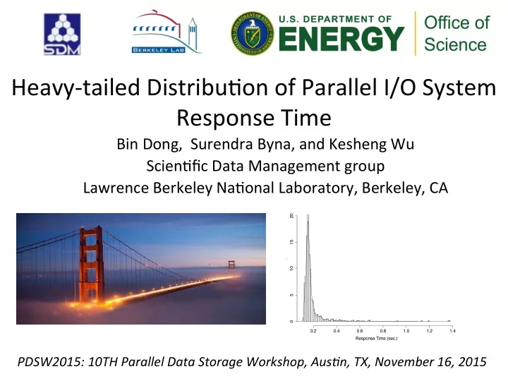
Outline ¡ • Mo1va1on ¡ • Response ¡1me ¡sampling ¡method ¡ • Analysis ¡results ¡of ¡response ¡1me ¡ ¡ ¡

Es1ma1ng ¡Response ¡Time ¡of ¡I/O ¡is ¡Essen1al ¡Element ¡ • Data ¡analysis ¡query ¡plan ¡op1mizing ¡ ¡ – Choose ¡index ¡or ¡data ¡organiza1on ¡with ¡minimum ¡ read ¡1me ¡ – Scien1fic ¡Data ¡Services ¡(SDS) ¡framework, ¡ ¡ PostgresSQL, ¡SciDB ¡ • Data ¡wri1ng ¡performance ¡tuning ¡ – Select ¡striping ¡size, ¡striping ¡account, ¡and ¡other ¡ parameters ¡to ¡reduce ¡write ¡1me ¡ – ExaHDF5, ¡I/O ¡Scheduler ¡ • Simulator, ¡ ¡Job ¡Scheduler ¡, ¡Quality ¡of ¡service ¡(QoS), ¡etc. ¡ ¡

Modeling ¡Response ¡Time ¡for ¡Parallel ¡I/O ¡ Response ¡1me ¡of ¡a ¡single ¡big ¡file ¡request ¡R: ¡ ¡ ¡ ¡ ¡ ¡T ¡= ¡max ¡(t 1 ¡ , ¡t 2 ¡ , ¡ ¡. ¡. ¡. ¡, ¡ ¡t n ¡) ¡+ ¡μ ¡ ¡ R ¡ ¡ ¡ ¡ ¡ ¡ ¡Split ¡overhead, ¡ ¡ ¡ ¡ ¡write ¡ . ¡. ¡. ¡ T ¡ μ ¡= ¡ ¡ Merge ¡overhead, ¡ ¡ ¡ ¡ ¡ ¡read ¡ t 1 ¡ t n ¡ t 2 ¡ t 1 ¡, ¡t 2 ¡, ¡. ¡. ¡., ¡t n: ¡ response ¡1mes ¡ of ¡ n ¡small ¡requests ¡ r 1 ¡ r 2 ¡ r n ¡ . ¡. ¡. ¡ I/O ¡Servers ¡in ¡PFS ¡ (e.g., ¡OST ¡in ¡Lustre) ¡

Simplifying ¡Response ¡Time ¡Model ¡ . ¡. ¡. ¡ T ¡= ¡max ¡(t 1 ¡ , ¡t 2 ¡ , ¡ ¡. ¡. ¡. ¡, ¡ ¡t n ¡) ¡+ ¡μ ¡ ¡ T ¡ t 1 ¡ t n ¡ . ¡. ¡. ¡ • Split/merge ¡overhead ¡ ¡μ ¡ is ¡constant ¡ ¡ • n ¡small ¡requests ¡ ¡ ¡ ≈ ¡ ¡ ¡ n ¡sampling ¡( i.i.d. ) ¡of ¡ n ¡IO ¡Servers ¡ • t 1 , ¡…, ¡t n ¡ ¡ ≈ ¡ ¡ ¡ n ¡ ¡ i.i.d. ¡sta1s1cal ¡variables ¡ • Focus ¡study ¡on ¡one ¡(denoted ¡by ¡ t) ¡among ¡ t 1 , ¡…, ¡t n ¡ ¡ ¡ – t ¡ : ¡ ¡con1nuously ¡distributed ¡variable ¡on ¡ (0, ¡ ¡+∞) ¡

Applying ¡Order ¡Sta1s1cs ¡to ¡Es1mate ¡ T ¡ T ¡ ¡= ¡ ¡maximum ¡(t 1 , ¡. ¡. ¡. ¡, ¡ ¡t n ¡) ¡+ ¡μ ¡ ¡ ¡ ¡ ¡ ¡ ¡ ¡ ¡ ¡ ¡ ¡ ¡ ¡ ¡ ¡ ¡ ¡ ¡ ¡t ¡ ¡: ¡ ¡ ¡con1nuously ¡distributed ¡variable ¡on ¡ (0, ¡ ¡+∞) ¡ ¡ ¡ ¡ ¡ ¡ ¡ ¡ ¡ ¡ ¡ ¡ ¡ ¡F t (x) ¡ : ¡ ¡ ¡distribu1on ¡func1on ¡of ¡ t ¡ ¡ ¡ f t (x) ¡= ¡F t ¡ ’ (x) ¡: ¡ ¡ ¡density ¡func1on ¡of ¡ t ¡ ¡ ¡ • Step ¡1 ¡ : ¡ ¡ ¡Compute ¡density ¡func1on ¡ f Yi (y) ¡with ¡ F t (x) ¡and ¡f t (x) ¡ ¡ – ¡Y i ¡ : ¡ ¡ the ¡ i-­‑ th ¡ largest ¡value ¡ ¡ (t 1 , ¡t 2 , ¡ ¡…, ¡ ¡t n ) ¡ Order ¡ ¡ Sta1s1cs ¡ ¡ – ¡f Yi (y) ¡ ¡= ¡F(y) n-­‑i (1-­‑F(y)) n-­‑i ¡f t (y) ¡n!/[(i-­‑1)!(n-­‑i)!] ¡ ¡ • Step ¡2 ¡ : ¡ ¡ ¡Compute ¡response ¡1me ¡ T ¡= ¡Y n ¡ ¡

Problem ¡Statement ¡ • What ¡is ¡the ¡distribu1on ¡func1on ¡ F(t) ¡for ¡the ¡ response ¡1me ¡of ¡each ¡small ¡file ¡request? ¡ – Exis1ng ¡researches ¡assume ¡ • Uniform ¡Distribu1on ¡ • Normal ¡Distribu1on ¡ – Are ¡these ¡assump1ons ¡true ¡? ¡ – If ¡not, ¡are ¡there ¡other ¡distribu1ons ¡fi^ng ¡be_er ¡? ¡ ¡ ¡ ¡ ¡

Our ¡Method ¡ • Sample ¡the ¡response ¡1me ¡of ¡two ¡produc1on ¡ storage ¡systems ¡ ¡ • Analyze ¡sta1s1cal ¡proper1es ¡of ¡response ¡1me ¡

Response ¡Time ¡Sampling ¡Environments ¡ • Hopper ¡and ¡Edison ¡at ¡NERSC 1 ¡ – 153K ¡and ¡130K ¡ ¡ CPU ¡cores, ¡ 1.28 ¡ PF ¡and ¡ 2.39 PF ¡ – 5000 ¡registered ¡users ¡ ¡ Compu1ng ¡Node ¡ /w ¡Lustre ¡Client ¡ – 300 ¡online ¡ac1ve ¡users ¡on ¡Edison ¡ – I/O ¡Intensive ¡jobs ¡use ¡Lustre ¡ ¡ Cache ¡ • Lustre ¡file ¡system ¡ – Cache ¡on ¡client ¡and ¡I/O ¡server ¡ Network ¡Router ¡ – Network ¡latency ¡ – 1 ¡~ ¡143 ¡OSTes ¡ ¡ Cache ¡ 1 Na;onal ¡Energy ¡Research ¡Scien;fic ¡Compu;ng ¡Center ¡ Lustre ¡OST ¡ ¡ ¡haps://www.nersc.gov/ ¡ ¡ ¡

Sampling ¡Method ¡ • One ¡job ¡sampling ¡one ¡OST ¡ – A ¡job ¡ ¡ ≈ ¡ ¡A ¡small ¡file ¡request ¡ – Measure ¡1me ¡of ¡reading ¡and ¡wri1ng ¡separately ¡ – Test ¡different ¡reading/wri1ng ¡sizes ¡ • 12 ¡different ¡sizes: ¡512KB, ¡1MB, ¡2MB, ¡ ¡… ¡, ¡1024MB ¡ – Match ¡request ¡size ¡and ¡striping ¡size ¡ ≈ ¡Job ¡ t ¡

Sampling ¡Method ¡ • Measure ¡response ¡1me ¡on ¡compu1ng ¡node ¡ – network, ¡disk, ¡cache ¡ • Cache ¡Considera1on ¡ Compu1ng ¡Node ¡ /w ¡Lustre ¡Client ¡ – No ¡Cache ¡ • clear ¡cache ¡by ¡accessing ¡memory ¡ ¡ Cache ¡ ¡ ¡ ¡ ¡sized ¡data ¡before ¡sampling ¡ ¡ • call ¡fsync() ¡ager ¡write ¡ Network ¡Router ¡ – Cache ¡ ¡ • High ¡frequently ¡sampling ¡ ¡ Cache ¡ Lustre ¡OST ¡

Sampling ¡Results ¡Sta1s1cs ¡Overview ¡ Start ¡Time ¡ End ¡Time ¡ Days ¡ # ¡of ¡ # ¡of ¡ ¡ Sampling ¡ OSTs ¡ Edison-­‑ ¡ 08/13/2014 ¡ 09/17/2014 ¡ 35 ¡ 14,977 ¡ 12 ¡ No-­‑Cache ¡ Edison-­‑ 02/20/2015 ¡ 02/20/2015 ¡ 1 ¡ 927,691 ¡ 12 ¡ Cache ¡ Hopper-­‑ ¡ 10/01/2014 ¡ 01/13/2015 ¡ 104 ¡ 13,868 ¡ 12 ¡ No-­‑Cache ¡ Hopper-­‑ 02/20/2015 ¡ 02/20/2015 ¡ 1 ¡ 1,581,364 ¡ 12 ¡ Cache ¡ Summary ¡ 141 ¡ 2,537,900 ¡ 48 ¡

Variability ¡of ¡Raw ¡Response ¡Time ¡for ¡ ¡ Edison ¡and ¡Hopper, ¡Cache ¡and ¡No-­‑Cache ¡

Ill-­‑fit ¡of ¡Uniform ¡or ¡Normal ¡Distribu1on ¡ Uniform ¡ ¡ Uniform ¡ ¡ Normal ¡ ¡ Normal ¡ ¡ Response ¡ ¡ Response ¡ ¡ 1me ¡of ¡different ¡ ¡ 1me ¡of ¡different ¡ ¡ request ¡sizes ¡ ¡ request ¡sizes ¡ ¡ Metrics ¡ ¡ Uniform ¡ Normal ¡ Kurtosis ¡ -­‑ ¡1.2 ¡ 3 ¡ Skewness ¡ 0 ¡ 0 ¡

Ill-­‑fit ¡of ¡Uniform, ¡Normal, ¡ ¡and ¡Other ¡Single ¡ Distribu1on ¡Func1on ¡ Read (Stripe Size: 64MB) 20 Single ¡distribu1on ¡func1ons ¡ • Power ¡Law ¡ ¡ ¡ Characters ¡of ¡Histogram: ¡ • Weibull ¡ 15 • A ¡single ¡peak ¡ • Exponen1al ¡ ¡ Histogram ¡ • Log ¡Normal ¡ ¡ Probability • Nonsymmetrical ¡ ¡ • Gamma ¡ 10 • Tail ¡is ¡real ¡long ¡ ¡ • Normal ¡ • Cauchy ¡ • Uniform ¡ 5 don’t ¡fit ¡very ¡well ¡! ¡ 0 0.2 0.4 0.6 0.8 1.0 1.2 1.4 Response Time (sec.)

Exploring ¡New ¡Distribu1ons ¡ • Par11on ¡response ¡1me ¡into ¡Head ¡and ¡Tail ¡ • Find ¡the ¡pivot ¡ – minimizing ¡KS ¡(Kolmogorov-­‑Smirnov) ¡distances ¡ • Normal ¡ • Cauchy ¡ Histogram ¡ ¡ Histogram ¡ • Power ¡Law ¡ • Weibull ¡ Histogram ¡ • Exponen1al ¡ • Log ¡Normal ¡ • Gamma ¡

Fi^ng ¡Results ¡ • Edison–NoCache, ¡ ¡Read ¡Response ¡Time, ¡ ¡64MB ¡ Accuracy ¡ ¡ Head ¡Group ¡ Normal ¡> ¡Cauchy ¡ Tail ¡Group ¡ Power ¡Law ¡> ¡Log ¡Normal ¡> ¡Exponen1al ¡> ¡Weibull ¡> ¡Gamma ¡ ¡

Fi^ng ¡Results ¡ • Edison–NoCache, ¡ ¡Write ¡Response ¡Time, ¡64MB ¡ Accuracy ¡ ¡ Head ¡Group ¡ Normal ¡> ¡Cauchy ¡ Tail ¡Group ¡ Power ¡Law ¡> ¡Weibull ¡> ¡Exponen1al ¡> ¡Log ¡Normal ¡> ¡Gamma ¡

Percentage ¡of ¡Head ¡group ¡and ¡Tail ¡group ¡ • 85% ¡in ¡Head ¡group ¡(i.e., ¡small ¡response ¡1me) ¡ • 15% ¡in ¡Tail ¡group ¡(i.e., ¡long ¡response ¡1me) ¡