H ( z ) x ( t ) CT DT DT CT y ( t ) X ( j ) X (e j ) X i ( j ) T - PowerPoint PPT Presentation

Overview of Sampling Topics Amplitude versus Time • (Shannon) sampling theorem • In this class we are working only with continuous-valued signals • Impulse-train sampling • Signals with discrete values that have been quantized are called digital signals • Interpolation (continuous-time signal reconstruction) • Analog-to-Digital converters (ADC) convert continuous-valued • Aliasing signals to discrete-valued signals. These often also convert from • Relationship of CTFT to DTFT CT to DT. • DT processing of CT signals • Digital-to-analog converters (DAC) convert discrete-valued signals to continuous-valued signals. These often also convert • DT sampling from DT to CT. • Decimation & interpolation • Signals that are both continuous-valued and continuous-time are usually called analog signals • Signals that are both discrete-valued and discrete-time are usually called digital J. McNames Portland State University ECE 223 Sampling Ver. 1.15 1 J. McNames Portland State University ECE 223 Sampling Ver. 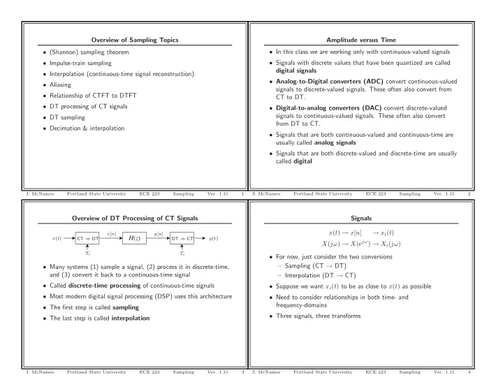1.15 2 Overview of DT Processing of CT Signals Signals x ( t ) → x [ n ] → x i ( t ) x [ n ] y [ n ] H ( z ) x ( t ) CT ⇒ DT DT ⇒ CT y ( t ) X ( jω ) → X (e jω ) → X i ( jω ) T s T s • For now, just consider the two conversions – Sampling (CT → DT) • Many systems (1) sample a signal, (2) process it in discrete-time, and (3) convert it back to a continuous-time signal – Interpolation (DT → CT) • Called discrete-time processing of continuous-time signals • Suppose we want x i ( t ) to be as close to x ( t ) as possible • Most modern digital signal processing (DSP) uses this architecture • Need to consider relationships in both time- and frequency-domains • The first step is called sampling • Three signals, three transforms • The last step is called interpolation J. McNames Portland State University ECE 223 Sampling Ver. 1.15 3 J. McNames Portland State University ECE 223 Sampling Ver. 1.15 4

Guiding Questions and Objectives Need for a Bridge Signal Consider three signals x [ n ] = x ( t ) | t = nT s Type Time Domain Frequency Domain Original Signal CT x ( t ) X ( jω ) X (e j Ω ) • The operation of sampling (CT → DT conversion) is trivial Sampled Signal DT x [ n ] Bridge Signal CT x δ ( t ) X δ ( jω ) • The challenge is to understand the limits and tradeoffs • Goals: to determine the relationship of x ( t ) to x [ n ] = x ( nT s ) in • The remainder of these slides is dedicated to answering the the time and frequency domains following three questions • In the time domain, the relationship x [ n ] = x ( nT s ) is clear 1. How is the CTFT of x ( t ) , X ( jω ) related to the DTFT of x [ n ] = x ( nT s ) , X (e j Ω ) ? • But what is the relationship of X ( jω ) to X (e j Ω ) ? 2. Under what conditions can we synthesize x ( t ) from x [ n ] : • The transforms differ in character x [ n ] → x ( t ) ? – X (e j Ω ) is periodic 3. How do we perform this DT → CT conversion? – X (e j Ω ) has units of radians per sample • A bridge signal x δ ( t ) is the only way (that I know of) to determine how X ( jω ) is related to X (e j Ω ) J. McNames Portland State University ECE 223 Sampling Ver. 1.15 5 J. McNames Portland State University ECE 223 Sampling Ver. 1.15 6 Use of the Bridge Signal Defining the Bridge Signal • Define the bridge signal by relating X δ ( jω ) to X (e j Ω ) • The bridge signal x δ ( t ) is a CT representation of a DT signal x [ n ] • It is defined as having the same transform, within a scale factor, • Determine how x ( t ) is related to x δ ( t ) in the time domain as the DT signal • Determine how X ( jω ) is related to X δ ( jω ) • Suppose x [ n ] = A e j (Ω n + φ ) • Use the relationships of X (e j Ω ) and X ( jω ) to X δ ( jω ) to • What is the CT equivalent? determine their relationship to one another • Let us pick x ( t ) = A e j ( ωt + φ ) • How do we relate the DT frequency Ω to the CT frequency ω ? – ω has units of radians/second – Ω has units of radians/sample • Let us use the conversion factor of T s = f − 1 seconds/sample s Ω (radians/sample) = ω (radians/second) × T s (seconds/sample) ω (radians/second) = Ω (radians/sample) × f s (samples/second) J. McNames Portland State University ECE 223 Sampling Ver. 1.15 7 J. McNames Portland State University ECE 223 Sampling Ver. 1.15 8

Defining the Bridge Signal Solving for the Bridge Signal X δ ( jω ) = X (e j Ω ) Ω= ωT s = X (e jωT s ) � ∞ � X (e j Ω ) = � x [ n ] e − j Ω n • The bridge signal is a CT representation of a DT signal n = −∞ ∞ • We define it by equating the CTFT and DTFT with an � X δ ( jω ) = X (e j Ω ) � x [ n ] e − jωT s n Ω= ωT s = � appropriate scaling factor for frequency n = −∞ • Note that this is a highly unusual CT signal FT x δ ( t ) ⇐ ⇒ X δ ( jω ) – The CTFT is periodic FT ⇒ e − jωt o δ ( t − t o ) ⇐ – What does this tell us about x δ ( t ) ? FT ⇒ e − jωT s n δ ( t − T s n ) ⇐ ∞ ∞ FT � � x [ n ] e − jωT s n x [ n ] δ ( t − T s n ) ⇐ ⇒ n = −∞ n = −∞ ∞ � x δ ( t ) = x [ n ] δ ( t − T s n ) n = −∞ J. McNames Portland State University ECE 223 Sampling Ver. 1.15 9 J. McNames Portland State University ECE 223 Sampling Ver. 1.15 10 Why Isn’t the Inverse Transform Similar to x ( t ) ? Impulse Sampling x [ n ] = 1 � X (e jω ) e j Ω n dΩ p ( t ) DTFT 1 2 π 2 π � + ∞ x ( t ) = 1 X ( jω ) e jωt d ω -4Ts -3Ts -2Ts -Ts 0 Ts 2Ts 3Ts 4Ts 5Ts CTFT 2 π −∞ ∞ � p ( t ) = δ ( t − nT s ) • We generated x δ ( t ) from x [ n ] by equating a CTFT to the DTFT of x [ n ] n = −∞ ∞ • This seems reasonable at first � x δ ( t ) = x ( nT s ) δ ( t − T s n ) = x ( t ) p ( t ) • But consider the range of the CTFT and DTFT synthesis n = −∞ equations • x δ ( t ) can also be formed from a CT signal • The DTFT synthesizes x [ n ] out of a finite range of frequencies • This is called impulse sampling • The CTFT synthesizes x ( t ) out of all frequencies • We can model sampling by use of the periodic impulse train • This is why, if x [ n ] = x ( nT s ) , that x δ ( t ) = F − 1 { X δ ( jω ) } = F − 1 � X (e jωT s ) � � = x ( t ) J. McNames Portland State University ECE 223 Sampling Ver. 1.15 11 J. McNames Portland State University ECE 223 Sampling Ver. 1.15 12

Rectangular Window and Impulse Train Notation Impulse Sampling Conceptual Example p ( t ) 1 x ( t ) 1 -4Ts -3Ts -2Ts -Ts 0 Ts 2Ts 3Ts 4Ts 5Ts • Note that a similar symbol was used for rectangular windows -4Ts -3Ts -2Ts -Ts 0 Ts 2Ts 3Ts 4Ts 5Ts � 1 | t | < T p ( t ) 1 p T ( t ) = 0 Otherwise but p ( t ) � = p T ( t ) -4Ts -3Ts -2Ts -Ts 0 Ts 2Ts 3Ts 4Ts 5Ts x ( t ) p ( t ) 1 -4Ts -3Ts -2Ts -Ts 0 Ts 2Ts 3Ts 4Ts 5Ts J. McNames Portland State University ECE 223 Sampling Ver. 1.15 13 J. McNames Portland State University ECE 223 Sampling Ver. 1.15 14 Impulse Sampling Terminology Fourier Transforms of Periodic Signals Overview ∞ x [ n ] y [ n ] � x δ ( t ) = x ( nT s ) δ ( t − T s n ) = x ( t ) p ( t ) H ( z ) x ( t ) CT ⇒ DT DT ⇒ CT y ( t ) n = −∞ X δ ( jω ) = 1 T s T s 2 π X ( jω ) ∗ P ( jω ) ∞ • To determine how X δ ( jω ) is related to X ( jω ) , we need to � x δ ( t ) = x ( t ) p ( t ) = x ( nT s ) δ ( t − nT s ) calculate P ( jω ) n = −∞ • p ( t ) is a periodic function with infinite energy • The impulse train p ( t ) is called the sampling function • The CTFT clearly doesn’t converge • p ( t ) is periodic with fundamental period T s • Is easier to • T s , the fundamental period of p ( t ) , is called the sampling period – Calculate the Fourier series coefficients P [ k ] for p ( t ) T s and ω s = 2 π 1 – Solve for P ( jω ) from P [ k ] using the general relationship • f s ≡ T s are called the sampling frequency between the CTFS and the CTFT • Since periodic signals have infinite energy, the CTFT of these signals consists of impulses J. McNames Portland State University ECE 223 Sampling Ver. 1.15 15 J. McNames Portland State University ECE 223 Sampling Ver. 1.15 16

Fourier Transforms of Periodic Signals Example 1: CT Fourier Transform of an Impulse Train Recall the Fourier series representations of periodic signals Solve for the Fourier transform of the impulse train ∞ ∞ � � X [ k ] e jkωt x ( t ) = p ( t ) = δ ( t − nT s ) k = −∞ n = −∞ FT e jω o t Hint: the impulse train is periodic. ⇐ ⇒ 2 π δ ( ω − ω o ) ∞ ∞ � + ∞ X [ k ] = 1 � FT x ( t )e − jkω o t d t x ( t ) e − jωt d t � X [ k ] e jkω o t � x ( t ) = ⇐ ⇒ 2 π X [ k ] δ ( ω − kω o ) X ( jω ) = T T −∞ k = −∞ k = −∞ J. McNames Portland State University ECE 223 Sampling Ver. 1.15 17 J. McNames Portland State University ECE 223 Sampling Ver. 1.15 18 Example 1: Workspace The Relationship of X ( jω ) to X δ ( jω ) 1 FT x ( t ) p ( t ) ⇐ ⇒ 2 π X ( jω ) ∗ P ( jω ) ∞ 2 π � � FT � ω − k 2 π P ( jω ) ⇐ ⇒ δ T s T s k = −∞ 2 π � ω s T s ∞ 2 π X ( jω ) ∗ 2 π 1 FT � x ( t ) p ( t ) ⇐ ⇒ δ ( ω − kω s ) T s k = −∞ X ( jω ) ∗ δ ( ω − ω o ) = X ( j ( ω − ω o )) ∞ 1 FT � x ( t ) p ( t ) ⇐ ⇒ X ( j ( ω − kω s )) T s k = −∞ J. McNames Portland State University ECE 223 Sampling Ver. 1.15 19 J. McNames Portland State University ECE 223 Sampling Ver. 1.15 20