h ( t ) y ( t ) Several derivations of the convolution integral - - PowerPoint PPT Presentation

h t
SMART_READER_LITE
LIVE PREVIEW

h ( t ) y ( t ) Several derivations of the convolution integral - - PowerPoint PPT Presentation

Overview of Convolution Integral Topics Impulse Response Impulse response defined x ( t ) h ( t ) y ( t ) Several derivations of the convolution integral Relationship to circuits and LTI systems Recall that if x ( t ) = ( t ) ,


slide-1
SLIDE 1

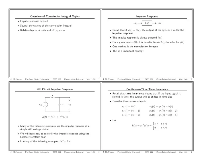
RC Circuit Impulse Response

C R

  • +

x(t) y(t)

h(t) = RC · e−

t RC u(t)

  • Many of the following examples use the impulse response of a

simple RC voltage divider

  • We will learn how to solve for this impulse response using the

Laplace transform soon

  • In many of the following examples RC = 1 s
  • J. McNames

Portland State University ECE 222 Convolution Integral

  • Ver. 1.68

3

Overview of Convolution Integral Topics

  • Impulse response defined
  • Several derivations of the convolution integral
  • Relationship to circuits and LTI systems
  • J. McNames

Portland State University ECE 222 Convolution Integral

  • Ver. 1.68

1

Continuous-Time Time Invariance

  • Recall that time invariance means that if the input signal is

shifted in time, the output will be shifted in time also

  • Consider three separate inputs

x1(t) = δ(t) x1(t) → y1(t) = h(t) x2(t) = δ(t − 2) x2(t) → y2(t) = h(t − 2) x3(t) = δ(t − 5) x3(t) → y3(t) = h(t − 5)

  • Let

h(t) = e−tu(t) =

  • e−t

t > 0 t < 0

  • J. McNames

Portland State University ECE 222 Convolution Integral

  • Ver. 1.68

4

Impulse Response h(t)

x(t) y(t)

  • Recall that if x(t) = δ(t), the output of the system is called the

impulse response

  • The impulse response is always denoted h(t)
  • For a given input x(t), it is possible to use h(t) to solve for y(t)
  • One method is the convolution integral
  • This is a important concept
  • J. McNames

Portland State University ECE 222 Convolution Integral

  • Ver. 1.68

2

slide-2
SLIDE 2

Input Decomposition Let x(t) = r(t) − 2 · r(t − 1) + ·r(t − 2) = ⎧ ⎪ ⎨ ⎪ ⎩ t 0 ≤ t ≤ 1 −(t − 2) 1 ≤ t ≤ 2

  • therwise
  • We can approximate any bounded signal x(t) as a series of pulses

with width w and height proportional to x(t) x(t) ≈

  • k=−∞

x(kw)

  • u
  • t − (k − 1

2)w

  • − u
  • t − (k + 1

2)w

  • J. McNames

Portland State University ECE 222 Convolution Integral

  • Ver. 1.68

7

Example 1: Continuous-Time Time Invariance

−2 2 4 6 8 10 0.5 1 x1(t) = δ(t−0) Input −2 2 4 6 8 10 0.5 1 y1(t) = h(t−0) Output −2 2 4 6 8 10 0.5 1 x2(t) = δ(t−2) −2 2 4 6 8 10 0.5 1 y2(t) = h(t−2) −2 2 4 6 8 10 0.5 1 x3(t) = δ(t−5) Time (s) −2 2 4 6 8 10 0.5 1 y3(t) = h(t−5) Time (s)

  • J. McNames

Portland State University ECE 222 Convolution Integral

  • Ver. 1.68

5

Example 2: Input Decomposition

−0.5 0.5 1 1.5 2 2.5 0.5 1 Input x(t) −0.5 0.5 1 1.5 2 2.5 0.5 1 w = 0.50 −0.5 0.5 1 1.5 2 2.5 0.5 1 w = 0.25 −0.5 0.5 1 1.5 2 2.5 0.5 1 w = 0.10 −0.5 0.5 1 1.5 2 2.5 0.5 1 w = 0.04 Time (s)

  • J. McNames

Portland State University ECE 222 Convolution Integral

  • Ver. 1.68

8

Example 1: MATLAB Code

t = -2:0.001:10; tc = [0 2 5]; for c1 = 1:length(tc), subplot(length(tc),2,c1*2-1); h = plot(tc(c1)*[1 1],[0 1],’b’,tc(c1),0.95,’b^’); set(h,’MarkerFaceColor’,’b’); set(h,’MarkerSize’,3); st = sprintf(’x_%d(t) = \\delta(t-%d)’,c1,tc(c1)); disp(st) ylabel(st); box off; xlim([min(t) max(t)]); ylim([0 1]); subplot(length(tc),2,c1*2); y1 = exp(-(t-tc(c1))).*(t>=tc(c1)); % Unit impulse response h[n] h = plot(t,y1,’r’); st = sprintf(’y_%d(t) = h(t-%d)’,c1,tc(c1)); ylabel(st); box off; xlim([min(t) max(t)]); end;

  • J. McNames

Portland State University ECE 222 Convolution Integral

  • Ver. 1.68

6

slide-3
SLIDE 3

Example 3: RC Pulse Response

−2 2 4 6 8 10 0.2 0.4 Input x(t) −2 2 4 6 8 10 0.5 1 Output y(t) h(t) y(t) −2 2 4 6 8 10 0.5 1 Input x(t) −2 2 4 6 8 10 0.5 1 Output y(t) h(t) y(t) −2 2 4 6 8 10 5 10 Input x(t) Time (s) −2 2 4 6 8 10 0.5 1 Output y(t) Time (s) h(t) y(t)

  • J. McNames

Portland State University ECE 222 Convolution Integral

  • Ver. 1.68

11

Example 2: MATLAB Code

fs = 1000; t0 = -0.5; t1 = 2.5; h = [0.50 0.25 0.10 0.04]; subplot(length(h)+1,1,1); t = t0:1/fs:t1; x = t.*(t>=0&t<1) + (-(t-2)).*(t>=1&t<2); hp = plot(t,x); set(hp,’MarkerFaceColor’,’b’); set(hp,’MarkerSize’,3); title(’Input’); ylabel(’x(t)’); box off; xlim([t0 t1]); for c1 = 1:length(h), subplot(length(h)+1,1,c1+1); t = t0:h(c1):t1; x = t.*(t>=0&t<1) + (-(t-2)).*(t>=1&t<2); hp = bar(t,x,1); set(hp,’FaceColor’,’w’); set(hp,’EdgeColor’,’r’); st = sprintf(’w = %4.2f’,h(c1)); ylabel(st); box off; xlim([t0 t1]); end;

  • J. McNames

Portland State University ECE 222 Convolution Integral

  • Ver. 1.68

9

Example 3: MATLAB Code

sys = tf([0 1],[1 1]); % Transfer function of an RC circuit with RC = 1 t = -2:0.001:10; ht = exp(-t).*(t>=0); % System impulse response h = [2.0 1.0 0.1]; for c1 = 1:length(h), subplot(length(h),2,(c1-1)*2+1); x = (t>0 & t<h(c1))/h(c1); plot(t,x); title(’Input’); ylabel(’x(t)’); box off; xlim([min(t) max(t)]); subplot(length(h),2,c1*2); y = lsim(sys,x,t); % Simulate the output of the system plot(t,ht,’g’,t,y,’r’); legend(’h(t)’,’y(t)’); title(’Output’); ylabel(’y(t)’); box off; xlim([min(t) max(t)]); end;

  • J. McNames

Portland State University ECE 222 Convolution Integral

  • Ver. 1.68

12

Replacing Rectangles with Impulses

  • If an input consists of a pulse that is sufficiently short in duration,

the continuous-time system will respond the same as it would to an impulse with the same area

  • The following example shows the response of an RC circuit to

three different pulses

  • Each pulse has unit area
  • The impulse response is also shown
  • Since the response is the same, we can replace our approximate

input signal that consists of rectangles with a train of impulses, if h is sufficiently small

  • J. McNames

Portland State University ECE 222 Convolution Integral

  • Ver. 1.68

10

slide-4
SLIDE 4

Example 4: MATLAB Code

fs = 1000; t0 = -0.5; t1 = 2.5; t = t0:1/fs:t1; x = t.*(t>=0&t<1) + (-(t-2)).*(t>=1&t<2); h = [0.5,0.25,0.10,0.04]; for c1 = 1:length(h), subplot(length(h),2,c1*2-1); th = t0:h(c1):t1; xr = th.*(th>=0&th<1) + (-(th-2)).*(th>=1&th<2); hb = bar(th,xr,1); set(hb,’FaceColor’,’w’); set(hb,’EdgeColor’,’b’); hold on; plot(t,x,’g’); hold off; st = sprintf(’w = %4.2f’,h(c1)); ylabel(st); box off; xlim([t0 t1]); subplot(length(h),2,c1*2); for c2 = 1:length(th), hp= plot(th(c2)*[1 1],[0 xr(c2)]*h(c1),’r’,th(c2),0.95*xr(c2)*h(c1),’r^’); hold on; set(hp(2),’MarkerFaceColor’,’r’); set(hp(2),’MarkerSize’,2); set(hp(2),’LineWidth’,0.001); end; hold off; box off; ylim([0 h(c1)]); xlim([t0 t1]); end;

  • J. McNames

Portland State University ECE 222 Convolution Integral

  • Ver. 1.68

15

Impulse Input Decomposition x(t) can approximated as a sum of pulses. x(t) = xr(t) =

  • k=−∞

w·x(kw)

  • u
  • t − (k − 1

2)w

  • − u
  • t − (k + 1

2)w

  • w

Each pulse can be approximated as a unit impulse δ(t − kw) = d u(t − kw) dt = lim

w→0

u

  • t − (k − 1

2)w

  • − u
  • t − (k + 1

2)w

  • w

so for small w, x(t) can also be approximated as a sum of impulses, x(t) ≈ xδ(t) =

  • k=−∞

w · x(kw) · δ(t − kw) Note that

−∞

δ(t − kw) dt =

−∞

  • u
  • t − (k − 1

2)w

  • − u
  • t − (k + 1

2)w

  • w

dt = 1

  • J. McNames

Portland State University ECE 222 Convolution Integral

  • Ver. 1.68

13

Applying Linearity If x(t) ≈ xδ(t) =

  • k=−∞

w x(kw) δ(t − kw), then by linearity and time invariance, y(t) ≈ yδ(t) =

  • k=−∞

w x(kw) h(t − kw) In the limit as w → 0, if x(t) and y(t) are integrable, we have x(t) = lim

w→0 xδ(t) =

−∞

x(τ) δ(t − τ) dτ y(t) = lim

w→0 yδ(t) =

−∞

x(τ) h(t − τ) dτ This is the continuous-time convolution integral

  • J. McNames

Portland State University ECE 222 Convolution Integral

  • Ver. 1.68

16

Example 4: Approximations to x(t)

−0.5 0.5 1 1.5 2 2.5 0.5 1 w = 0.50 Approximation with Rectangles −0.5 0.5 1 1.5 2 2.5 0.5 Approximation with Impulses −0.5 0.5 1 1.5 2 2.5 0.5 1 w = 0.25 −0.5 0.5 1 1.5 2 2.5 0.1 0.2 −0.5 0.5 1 1.5 2 2.5 0.5 1 w = 0.10 −0.5 0.5 1 1.5 2 2.5 0.05 0.1 −0.5 0.5 1 1.5 2 2.5 0.5 1 w = 0.04 Time (s) −0.5 0.5 1 1.5 2 2.5 0.02 0.04 Time (s)

  • J. McNames

Portland State University ECE 222 Convolution Integral

  • Ver. 1.68

14

slide-5
SLIDE 5

Example 5: MATLAB Code Continued

subplot(length(ti)+1,2,length(ti)*2+1); for c1 = 1:length(ti), hp = plot(ti(c1)*[1 1],[0 xi(c1)]*h,’b’,ti(c1),0.95*xi(c1)*h,’b^’); set(hp,’MarkerFaceColor’,’b’); set(hp,’MarkerSize’,2); set(hp,’LineWidth’,0.001); hold on; end; hold off; box off; ylim([0 max(xi)*h]); xlim([min(t) max(t)]); xlabel(’Time (s)’); subplot(length(ti)+1,2,length(ti)*2+2); plot(t,yt,’g’,t,y,’r’); box off; ylim([0 0.66]); xlim([min(t) max(t)]); xlabel(’Time (s)’); legend(’True’,’Approximate’);

  • J. McNames

Portland State University ECE 222 Convolution Integral

  • Ver. 1.68

19

Example 5: Impulse Approximation and Output

−2 2 4 6 8 10 0.5 Input −2 2 4 6 8 10 0.5 Output −2 2 4 6 8 10 0.5 −2 2 4 6 8 10 0.5 −2 2 4 6 8 10 0.5 −2 2 4 6 8 10 0.5 −2 2 4 6 8 10 0.5 Time (s) −2 2 4 6 8 10 0.5 Time (s) True Approximate

  • J. McNames

Portland State University ECE 222 Convolution Integral

  • Ver. 1.68

17

Example 6: Approximate Outputs versus h

−2 2 4 6 8 10 0.2 0.4 Input −2 2 4 6 8 10 0.2 0.4 0.6 Output True Approximate −2 2 4 6 8 10 0.1 0.2 −2 2 4 6 8 10 0.2 0.4 0.6 True Approximate −2 2 4 6 8 10 0.05 0.1 Time (s) −2 2 4 6 8 10 0.2 0.4 0.6 Time (s) True Approximate

  • J. McNames

Portland State University ECE 222 Convolution Integral

  • Ver. 1.68

20

Example 5: MATLAB Code

sys = tf([0 1],[1 1]); % Transfer function of an RC circuit with RC = 1 t0 = -2; t1 = 10; t = t0:0.001:t1; xt = t.*(t>=0&t<1) + (-(t-2)).*(t>=1&t<2); % True system input yt = lsim(sys,xt,t); % Simulate the output of the system y = zeros(size(t)); h = 0.5; ti = [0.5 1.0 1.5]; % Impulse times xi = [0.5 1.0 0.5]*h; % Impulse Amplitudes for c1 = 1:length(ti), subplot(length(ti)+1,2,c1*2-1); hp= plot(ti(c1)*[1 1],[0 xi(c1)],’b’,ti(c1),0.95*xi(c1),’b^’); set(hp,’MarkerFaceColor’,’b’); set(hp,’MarkerSize’,2); set(hp,’LineWidth’,0.001); box off; ylim([0 max(xi)]); xlim([min(t) max(t)]); subplot(length(ti)+1,2,c1*2); yp = xi(c1)*exp(-(t-ti(c1))).*((t-ti(c1))>=0); % Response to a single impulse plot(t,yp,’r’); box off; ylim([0 0.66]); xlim([min(t) max(t)]); y = y + yp; % Total Response end;

  • J. McNames

Portland State University ECE 222 Convolution Integral

  • Ver. 1.68

18

slide-6
SLIDE 6

Convolution Integral Alternative Form y(t) = +∞

−∞

x(τ) h(t − τ) dτ Let u t − τ, then τ = t − u and dτ = −du. y(t) = −∞

x(t − u) h(u) (−du) = ∞

−∞

x(t − u) h(u) du = ∞

−∞

x(t − τ) h(τ) dτ

  • Both forms are called the convolution integral
  • This is often written as y(t) = x(t) ∗ h(t)
  • J. McNames

Portland State University ECE 222 Convolution Integral

  • Ver. 1.68

23

Example 6: MATLAB Code

sys = tf([0 1],[1 1]); % Transfer function of an RC circuit with RC = 1 t0 = -2; t1 = 10; t = t0:0.001:t1; x = t.*(t>=0&t<1) + (-(t-2)).*(t>=1&t<2); % True system input yt = lsim(sys,x,t); % Simulate the output of the system h = [0.50 0.25 0.10]; for c1 = 1:length(h), subplot(length(h),2,c1*2-1); th = t0:h(c1):t1; % Impulse times xr = th.*(th>=0&th<1) + (-(th-2)).*(th>=1&th<2); % Impulse amplitudes for c2 = 1:length(th), hp= plot(th(c2)*[1 1],[0 xr(c2)]*h(c1),’b’,th(c2),xr(c2)*h(c1),’b^’); hold on; set(hp,’MarkerFaceColor’,’b’); set(hp,’MarkerSize’,1.2); set(hp(1),’LineWidth’,0.3); set(hp(2),’LineWidth’,0.001); end; hold off; box off; subplot(length(h),2,c1*2); y = zeros(size(t)); for c2 = 1:length(th), y = y + h(c1)*xr(c2)*exp(-(t-th(c2))).*((t-th(c2))>=0); end; hp = plot(t,yt,’g’,t,y,’r’); set(hp(1),’LineWidth’,0.8); set(hp(2),’LineWidth’,0.3); legend(’True’,’Approximate’); box off; end;

  • J. McNames

Portland State University ECE 222 Convolution Integral

  • Ver. 1.68

21

Intuition y(t) = x(t) ∗ h(t) = +∞

−∞

x(τ) h(t − τ) dτ

  • Key point: The system output at t is in response to all past and

present values of the input signal, not just at time t

  • Conceptually, you can think of convolution as weighted averaging
  • The signal x(t) is being averaged
  • The impulse response h(t) determines how it is weighted
  • Lowpass filters tend to have smooth, slowly varying weights
  • Highpass and bandpass filters tend to be oscillatory
  • J. McNames

Portland State University ECE 222 Convolution Integral

  • Ver. 1.68

24

Continuous-Time Convolution Derivation Summary h(t) h(t) h(t) h(t)

Definition of h(t) Time Invariance Linearity

h(t)

Linearity

h(t) x(t) x(t) δ(t) δ(t − τ) x(τ) δ(t − τ) ∞

−∞ x(τ) δ(t − τ) dτ Definition of δ(t)

y(t) h(t) h(t − τ) x(τ) h(t − τ) ∞

−∞ x(τ) h(t − τ) dτ

−∞ x(τ) h(t − τ) dτ

  • J. McNames

Portland State University ECE 222 Convolution Integral

  • Ver. 1.68

22

slide-7
SLIDE 7

Summary h(t)

x(t) y(t)

y(t) = x(t)∗h(t) = +∞

−∞

x(t−τ) h(τ) dτ

  • The convolution integral describes how the output y(t) is related

to the input signal x(t) and the unit impulse h(t)

  • Only two assumptions were made about the system

– Linear – Time Invariant

  • Key points:

– The impulse response h(t) completely defines the behavior of continuous-time LTI systems – If h(t) is known, then the output of a continuous-time LTI system can be calculated for any input x(t) using the convolution integral

  • J. McNames

Portland State University ECE 222 Convolution Integral

  • Ver. 1.68

25