GTI Randomness and Probability A. Ada, K. Sutner Carnegie Mellon - - PDF document

gti randomness and probability
SMART_READER_LITE
LIVE PREVIEW

GTI Randomness and Probability A. Ada, K. Sutner Carnegie Mellon - - PDF document

GTI Randomness and Probability A. Ada, K. Sutner Carnegie Mellon University Spring 2018 Randomness 1 Probability Theory Total Recall 3 As you may remember fondly, you already saw an introduction to probability in 15-151: C. Newstead


slide-1
SLIDE 1

GTI Randomness and Probability

  • A. Ada, K. Sutner

Carnegie Mellon University Spring 2018

1

Randomness

  • Probability Theory

Total Recall

3

As you may remember fondly, you already saw an introduction to probability in 15-151:

  • C. Newstead & J. Mackey

An Infinite Descent Into Pure Mathematics

  • Chap. 7

This is the wilted stack of notes under your pillow . . .

slide-2
SLIDE 2

Battleplan

4

Next week we will discuss the use of randomness to speed up algorithms,

  • ne of the most important ideas in the theory of algorithms.

In preparation, this lecture is a gentle reminder to go back an re-read Chap. 7, if need be, and an attempt to explain some of the more foundational issues;

What The Hell Is Randomness?

5

Randomness is one of the most perplexing ideas in ToC: defining randomness in any mathematically correct way is very, very hard. Yet, any 6-year old knows very well from experience what randomness is: flipping a coin or rolling a die is a perfect example.

How Random Is It?

6

Is the randomness in a coin-toss real or is it actually confined to just the initial conditions? Persi Diaconis, a Stanford mathematician and highly accomplished professional magician, supposedly can consistently produce ten consecutive heads flipping a coin – by carefully controlling the initial conditions.

slide-3
SLIDE 3

Lava Lamps

7

Krypton-85

8

Radioactivity is another great source of randomness – except that no one likes to keep a lump of radioactive material and a Geiger-M¨ uller counter

  • n their desk. Solution: keep the radioactive stuff someplace else and get

the random bits over the web. True random bits from www.fourmilab.ch.

Huge Difference

9

The last system (and also the lava lamps, see below) is very different from the others: if our current understanding of physics is halfway correct, there is no way to predict certain events in quantum physics, like radioactive decay. It is fundamentally impossible (even if we could establish initial conditions correctly, which we cannot thanks to Herr Heisenberg). The other, purely mechanical systems such as dice and coins, we encounter deterministic chaos: given sufficiently precise descriptions of the initial conditions, and sufficient compute power, one could in principle compute the outcomes (if we think of them as classical systems). In principle only, not in practice.

slide-4
SLIDE 4

Lorenz Attractor

10

Here is a famous example discovered by Lorenz in the 1963, in an attempt to study a hugely simplified model of heat convection in the atmosphere. x′ = σ(y − x) y′ = rx − y − xz z′ = xy − bz These are not spatial coordinates, x stands for the amplitude of convective motion, y for temperature difference between rising and falling air currents, and z between temperature in the model and a simple linear approximation. For certain values of the parameters we get the following behavior.

Pre-History

12

In the olden days, the RAND Corporation used a kind of electronic roulette wheel to generate a million random digits (rate: one per second). In 1955 the data were published under the title: A Million Random Digits With 100,000 Normal Devi- ates “Normal deviates” simply means that the distribution of the random numbers is bell-shaped rather than uniform. But the New York Public Library shelved the book in the psychology section. The RAND guys were surprised to find that their original sequence had several defects and required quite a bit of post-processing before it could pass muster as a random sequence. This took years to do. Available at RAND.

slide-5
SLIDE 5

Fiat Lux

13

Incidentally, Noll and Cooper at Silicon Graphics discovered one day that the pretty lava lamps were completely irrelevant: they could get even better random bits with the lens cap on (there is enough noise in the circuits to get good randomness). Another way to use light, very much unlike the original lava lamp system, is to exploit an elementary quantum optical process: a photon hitting a semi-transparent mirror either passes or is reflected. The Quantis systems was developed at the University of Geneva, the first practical model was released in 1998. Note that quantum physics is the only part of physics that claims that the outcome of certain processes is fundamentally random (which is why Einstein was never very fond of quantum physics). See Idquantique.

The Magic Device

14

A true random number generator.

Quantis TRNG

15

Features True quantum randomness High bit rate, up to 16Mbits/sec Low-cost device (1000+ Euros) Compact and reliable USB or PCI, drivers for Windows and Linux Applications Numerical Simulations Statistical Research Lotteries and gambling Cryptography

slide-6
SLIDE 6

Hilbert’s 6th Problem

16

Mathematical Treatment of the Axioms of Physics. The investigations on the foundations of geometry suggest the problem: To treat in the same manner, by means of ax- ioms, those physical sciences in which already today math- ematics plays an important part; in the first rank are the theory of probabilities and mechanics. Kolmogorov axiomatized probability, but there is no hope for an axiomatic treatment of all of physics anywhere in the near future. It’s all poetry.

Some Don’t Mind

17

Is should be noted that even today not everyone participates in the quest for absolute Hilbertian precision. For example, physics super-star Steven Weinberg writes in a book on quantum field theory . . . there are parts of this book that will bring tears to the eyes of the mathematically inclined reader. In physics, this attitude may be a good thing that helps the field along. In ToC, it would more likely be an unmitigated disaster.

Random Sequences

18

It is somewhat easier to define what one means by an infinite random bit sequence rather than dealing with random finite sequences: α = a0, a1, a2, . . . , an, . . . ∈ 2ω Intuitively, what properties would we expect from a random α? Always think of α as being generated by infinitely many coin tosses. Of course, we want the coin to be fair. It is a really obnoxiuous question to ask what it means for a coin to be fair.

slide-7
SLIDE 7

Limiting Density

19

It is easy to define the density of a finite binary word x of length n: D(x) = 1/n

  • i

xi But how about an infinite sequence α?

Definition (Density)

Let α ∈ 2ω and define the density of α up to n to be D(α, n) = D(α[n]). The limiting density of α is D(α) = lim

n→∞ D(α, n)

Weinberg to the Rescue

20

Note that there is a huge problem with this definition: limits are precisely defined in analysis. But α is a wild-and-woolly object of our imagination, and there is not much reason to assume that this particular limit should exist. In fact, it does not always exist, but we will take the patented Weinberg Approach: fuggedaboudit.

The Law of Large Numbers

21

The LoLN says that if we repeat an experiment often, the observed average does in fact converge to the expected value; almost certainly. For example, for an unbiased coin we should expect to approach the limiting density of 1/2, almost always. Also note that we should not expect the averages to be exactly equal to the expectation. For example, performing a one-dimensional random walk with steps ±1 we should expect to be up to O(√n) from the origin after n steps.

slide-8
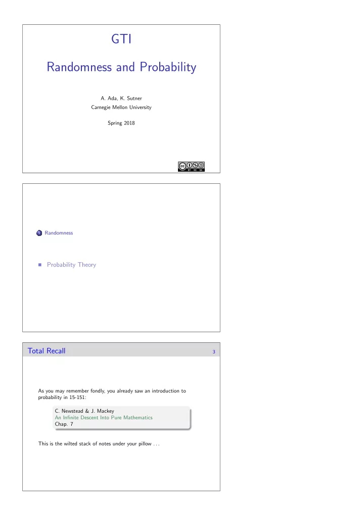
SLIDE 8

A Random Walk

22

200 400 600 800 1000 40 30 20 10 10 20

Decimation

23

How about using Roman military traditions to define randomness? In 1919 Richard von Mises suggested a notion of randomness based on the limiting density of the sequence itself and various decimations of it. The idea is that “reasonable” subsequences

  • f the given sequence should also have

limiting density 1/2.

Definition

An infinite sequence α ∈ 2ω is Mises random if the limiting density of any subsequence (aij) is 1/2 where the subsequence is selected by a Auswahlregel.

Auswahlregeln

24

So what on earth is a Auswahlregel, a selection rule? Intuitively, the following decimations all should have limiting density 1/2: a0, a1, a2, . . . , an, . . . a0, a2, a4, . . . , a2n, . . . a1, a4, a7, . . . , a3n+1, . . . a0, a1, a4, . . . , an2, . . . a2, a3, a5, . . . , a15485863, . . . In fact, we might want for any reasonable strictly monotonic function f : N → N that αf = af(0), af(1), af(2), . . . , af(n), . . . has limiting density 1/2.

slide-9
SLIDE 9

Mises’ Definition

25

However, there is one big caveat: the selector function f must be defined without any knowledge of α: otherwise we can simply pick a subsequence

  • f all 0’s or all 1’s.

Now suppose we have a countable system of Auswahlregeln and our sequence passes all these tests. In other words, for all f we have D(αf) = 1/2. Then α is Mises-random. One can show that for any countable collection

  • f Auswahlregeln there are always uncountably many sequences that are

random in this sense. Sounds all eminently reasonable.

Ville’s Counterexample

26

Unfortunately, in 1939 J. Ville showed that for any countable system of Auswahlregeln there is always a sequence α that passes all the tests (i.e., the limiting density is 1/2 for all these subsequences) but that is nonetheless biased towards 1. More precisely, it was known that a random sequence should have lim sup

n

  • 2n

log log n

  • D(α, n) − 1/2
  • = 1

lim inf

n

  • 2n

log log n

  • D(α, n) − 1/2
  • = −1

and Ville’s example violated the second condition.

Now What?

27

There are excellent definitions of randomness based on better tests. Instead of Auswahlregeln one uses tests with foundations in computability theory, and topology. The most famous one is due to Per Martin-L¨

  • f (who has also done

groundbreaking work in type theory). Following Weinberg’s proud example, we will forgo this opportunity to inflict mental pain and anguish on the student body, and skip over the definition.

slide-10
SLIDE 10

Randomness versus Computation

28

Unfortunately, all definitions of randomness have one unpleasant side-effect: random sequences are not computable. This is not a big surprise: computable means predictable, and we want exactly he opposite. Anyone attempting to produce random numbers by purely arithmetic means is, of course, in a state of sin. John von Neumann Mike Pence will object, but we have no problem with sin.

  • Randomness

2

Probability Theory

Discrete versus Continuous

30

Discrete Probability

  • Finite spaces: Really a matter of combinatorial counting, though

sometimes it is easier to argue in terms of probability.

  • Countably infinite spaces: Deals with infinite spaces and infinite

summations, but everything remains civilized.

Continuous Probability Uncountable spaces, really a part of measure theory, and annoyingly dependent on set theory. All hell breaks loose.

slide-11
SLIDE 11

Kolmogorov Axioms

31

The collection of all possible outcomes of an experiment is called a sample space Ω and its elements are the elementary events or atomic

  • events. A (compound) event is a subset of Ω.

We want to associate a probability for the occurrence of each event, a map Pr : P(Ω) → R 0 ≤ Pr[A] Pr[Ω] = 1 A ∩ B = ∅ implies Pr[A ∪ B] = Pr[A] + Pr[B]

What Could Go Wrong?

32

Discrete probability is pretty safe, but consider the following continuous problem: we would like to measure the area of regions in Euclidean space, something like µ(A) where A ⊆ Rd. This is closely related to probability theory: think about an experiment like throwing a dart at the unit square. What is the probability that the dart ends up in the region A below? Clearly we need to determine µ(A).

A Wishlist

33

For simplicity, consider d = 2. Norm We want µ(R) = ab whenever R is an a × b rectangle. Additivity (finite) If A = A1 ∪ . . . ∪ An then µ(A) ≤ µ(Ai). We have equality when the Ai are disjoint. Additivity (countable) If A =

i≥0 Ai then µ(A) ≤ µ(Ai).

We have equality when the Ai are disjoint. Invariance If B is congruent to A, then µ(A) = µ(B).

slide-12
SLIDE 12

Exclusive Events

34

The condition Ai ∩ Aj for i < j means that the events are mutually exclusive. No one doubts finite additivity, but countable additivity is also really quite natural: think about dividing the unit square into rectangles of size 2−n.

Lebesgue Measure

35

The now standard answer to the design of such a measure was given by Henri Lebesgue in 1902 in his dissertation: to measure a region A, approximate it by lots of rectangles (but in a non-obvious way).

No Luck

36

Theorem (Vitali 1905)

There are non-measurable sets of reals. This requires a little group theory and the Axiom of Choice. On the other hand, Solovay has constructed universes where all sets of reals are measurable. On the upside, there are finitely additive measures for d = 1, 2. Unfortunately, they fail to be unique.

Theorem (Hausdorff)

No finitely additive measures exist for d > 2.

slide-13
SLIDE 13

Now What?

37

The solution is quite natural: who cares about P(Rd)? The full power set is a weird monstrosity anyway, so why not restrict the measure to civilized subsets? The standard choice is Borel sets, sets that can be constructed from open sets by complements and countably unions. The Lebesgue measure works fine for Borel sets. As a practical matter, you will never encounter a subset of Rd that is not Borel (unless you are a logician and thrive on other people’s misery).

The Real World

38

Nowadays, CAS can automatically compute fairly complicated measures.

Even Symbolic

39

slide-14
SLIDE 14

Discrete Spaces

40

In the countably infinite case we have basic probabilities (pa)a∈Ω such that

a pa = 1.

As a consequence, we can can compute

a∈A pa for any A ⊆ Ω.

In fact, we can decompose everything into atomic events: Pr[A] =

  • a∈A

Pr[{a}] This fails miserably for uncountable spaces where Pr[{a}] = 0.

Back to Kolmogorov

41

In the Kolmogorov setup, ∅ is the impossible event, and Ω the certain event, with probabilities 0 and 1, respectively. The axioms have several easy consequences. 0 ≤ Pr[A] ≤ 1. Pr[A] = 1 − Pr[A]. A ⊆ B implies Pr[A] ≤ Pr[B]. The third axiom states additivity for two sets. By induction we immediately get full finite additivity: for any finite family of mutually exclusive events Pr[A1 ∪ A2 ∪ . . . ∪ Ak] = Pr[A1] + Pr[A2] + . . . + Pr[Ak].

More

42

How about general unions? Pr[A ∪ B] = Pr[A] + Pr[B] − Pr[A ∩ B] The last equation generalizes to unions of more than two terms, but is a bit clumsy to state (see the inclusion-exclusion principle in combinatorics). Bode’s Inequality: Pr[A1 ∪ A2 ∪ . . . ∪ Ak] ≤ Pr[A1] + Pr[A2] + . . . + Pr[Ak]. Bonferroni’s Inequality: Pr[A1 ∩ A2 ∩ . . . ∩ Ak] ≥ Pr[A1] + Pr[A2] + . . . + Pr[Ak] − (k − 1).

slide-15
SLIDE 15

Frequencies

43

In the discrete case, we only need to determine the elementary probabilities Pr[{a}] for all a ∈ Ω. One possibility is to axiomatically claim certain values. For example, for a finite space Ω we might declare uniform probabilities Pr[{a}] = 1/|Ω| Or we could try to measure them by repeating an experiment (often) and determining frequencies: Pr[{a}] = # successes # trials

Conditional Probability

44

Often one has additional information about the state of affairs that can affect the probability of some event A. This is captured by the notion of conditional probability: suppose Pr[B] > 0 and set Pr[A | B] = Pr[A ∩ B]/Pr[B] Sometimes one can partition Ω into exclusive events B1, . . . , Bk. Then we have Pr[A] =

  • Pr[A ∩ Bi] =
  • Pr[A | Bi] Pr[Bi]

The case k = 2 is often useful.

Independence

45

Here is the opposite idea: two events A and B are independent iff knowledge of one provides no information about the other. Pr[A ∩ B] = Pr[A] · Pr[B]

Exercise

Suppose A and B are independent. Show that A, B; A, B and A, B are all independent.

slide-16
SLIDE 16

Random Variables

46

Experiments are often associated with some numerical quantity, which depends on random outcomes: these thingies are random variables and defined as maps X : Ω → R Technically, in the continuous case we also need measurability of X−1(R≥r), but we won’t worry. The discrete case is always fine and it makes sense to talk about the probability distribution or probability mass function p(a) = Pr[X = a]

Why Reals?

47

Sometimes one would like to associate outcomes other than reals with an experiment, our definition of a random variable does not allow that. The reason is that reals are just too convenient. For example, nothing stops us from computing 5X2(a) + 3X(a) − 17 Or we could add RVs X(a) + Y (a) and so on. This will come in very handy.

Indicator Variables

48

We can fake other properties by choosing our random variables appropriately. For example, suppose we only care whether a ∈ A. This can be captured by an indicator variable X(a) =

  • 1

if a ∈ A,

  • therwise.
slide-17
SLIDE 17

Continuous Distributions

49

For continuous spaces we can still talk about the cumulative distribution function: p(a) = Pr[X ≤ a]

  • 6
  • 4
  • 2

2 4 6 0.2 0.4 0.6 0.8 1.0

Jumps

50

In the discrete case, the cdfs increase in steps.

2 4 6 8 10 0.2 0.4 0.6 0.8 1.0

In 3-D

51

slide-18
SLIDE 18

Expectation

52

Suppose we have a discrete random variable X with pmf p(a). The expected value or expectation of X is E[X] =

  • X(a) · p(a)

This is often abbreviated in slightly criminal manner to µ. So expectation is a weighted sum, and corresponds to the intuitive notion

  • f average.

Lemma

Expectation is linear in the sense that E[aX + bY ] = a E[X] + b E[Y ] where a and b are real constants.

Variance

53

Other than the average it is also useful to now how far off the values of a random variable might be, on average. The variance of X is Var[X] = E[(X − µ)2] This is often written as σ2 (where σ is the standard deviation). In other words, Var[X] = E[X2] − E[X]2.

Rules for Variance

54

Lemma

Var[aX + b] = a2Var[X].

Lemma

Assume that X and Y are independent. Then variance is additive in the sense that Var[X + Y ] = Var[X] + Var[Y ]. Incidentally, for independent variables we have Var[XY ] = Var[X] · Var[Y ].

slide-19
SLIDE 19

Chebyshev

55

Lemma (Chebyshev’s Inequality)

Suppose X has finite expectation µ and non-zero variance σ2. Then Pr[|X − µ| ≥ c] ≤ σ2/c2.

Uniform Distribution

56

A continuous variable X is uniformly distributed if for some interval [a, b] ⊆ R we have the pdf f(x) =

  • 1/(b − a)

if a ≤ x ≤ b,

  • therwise.

E[X] = (a + b)/2 Var[X] = (b − a)2/12

Finite Case

57

For a finite space Ω we similarly have Pr[X = a] = 1/|Ω| Just think about coins or dice. Dire Warning: this does not work for countably infinite spaces.

slide-20
SLIDE 20

Bernoulli

58

This is the distribution of an indicator variable with Pr[X = 1] = p E[X] = p Var[X] = p(1 − p)

Binomial

59

Define an indicator variable Xi that is 1 if the ith repetition produces the event, and 0 otherwise and consider X = X1 + X2 + . . . + Xn. If the probability of Xi is p then Pr[X = k] = n k

  • pk(1 − p)n−k

E[X] = np Var[X] = np(1 − p)

Geometric

60

If we count the number of times till heads appear we get a random variable X such that Pr[X = k] = p(1 − p)k−1 E[X] = 1/p Var[X] = (1 − p)/p2

slide-21
SLIDE 21

Normal

61

Parameters µ and σ. f(x) = 1 √ 2πσ e−(x−µ)2/(2σ2) E[X] = µ Var[X] = σ2

Bell Curve

62

  • 6
  • 4
  • 2

2 4 6 0.1 0.2 0.3 0.4 0.5

Experiments

63

  • 5

5 10 0.00 0.02 0.04 0.06 0.08 0.10 0.12

A lot of people spend a lot of time trying to match outcomes of experiments against a normal distribution.