Gray Level Modification Contrast Stretching (1) Underexposed - - PDF document

1

IIP 1

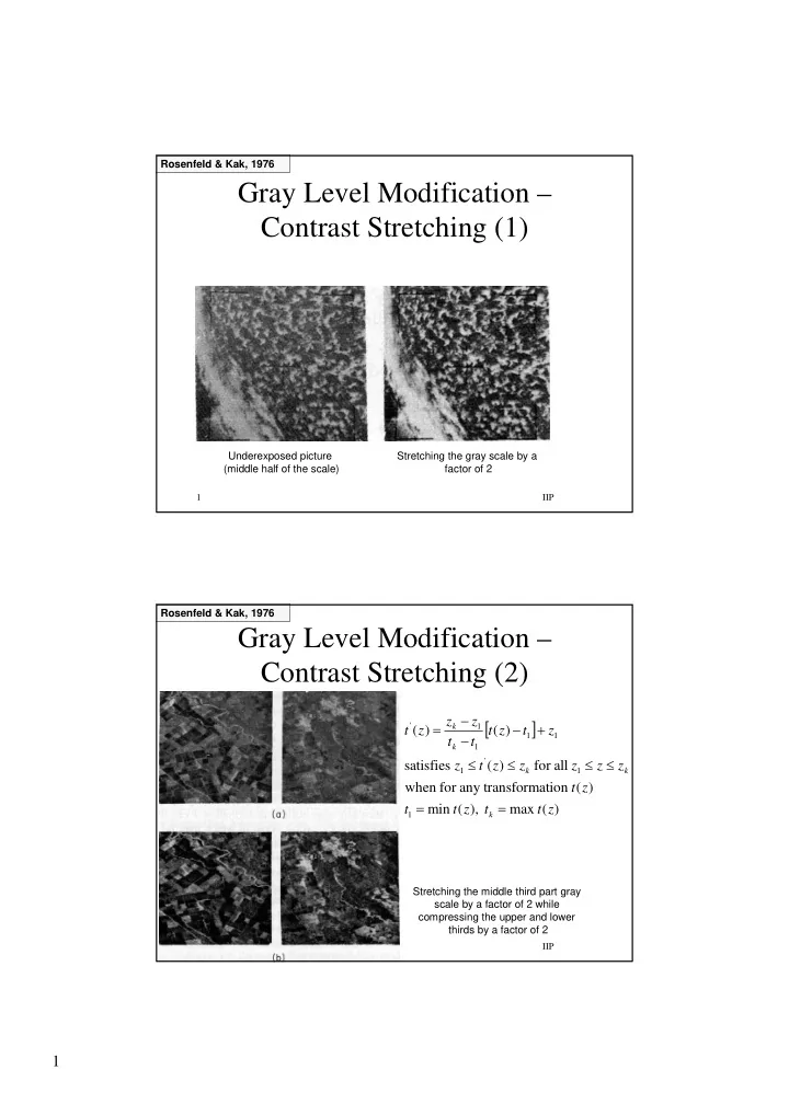
Gray Level Modification – Contrast Stretching (1)

Stretching the gray scale by a factor of 2 Underexposed picture (middle half of the scale) Rosenfeld & Kak, 1976

IIP 2

Gray Level Modification – Contrast Stretching (2)

Rosenfeld & Kak, 1976 Stretching the middle third part gray scale by a factor of 2 while compressing the upper and lower thirds by a factor of 2

[ ]

) ( max ), ( min ) (

• rmation

any transf for when all for ) ( satisfies ) ( ) (

1 1 ' 1 1 1 1 1 '

z t t z t t z t z z z z z t z z t z t t t z z z t

k k k k k

= = ≤ ≤ ≤ ≤ + − − − =

2

IIP 3

Histogram Matching (in comparison to

histogram equalization)

• Why having a uniform histogram for the output

image and not specifying a desired histogram?

[ ]

1 1

( ) ( ) ( ) ( ) ( ) ( )

r r z z

s T r p w dw G z p t dt s z G s G T r

− −

= = = = = =

∫ ∫

IIP 4

Image Enhancement – Agenda

• Algebraic/logic operations
• Geometric operations
• Image enhancement in the spatial domain

by filtering

3

IIP 5

Algebraic Operations

• Operated pixel-by-pixel

where A & B are the input images and C is the output image (and of course complex algebraic equations involving several images may be formed)

( , ) ( , ) ( , ) ( , ) ( , ) ( , ) ( , ) ( , ) x ( , ) ( , ) ( , ) ( , ) C x y A x y B x y C x y A x y B x y C x y A x y B x y C x y A x y B x y = + = − = = ÷

IIP 6

Uses of Algebraic Operations

• Addition

1) averaging multiple images of the same scene to reduce additive random noise 2) Superimposition of images (“double exposure”)

• Subtraction

1) remove additive pattern (background, periodic noise, additive contamination) 2) Change detection analysis 3) computing gradients for locating edges 4) motion detection

• Multiplication & Division – less applicative

4

IIP 7

Applications of Algebraic Operations

• Averaging for noise reduction (multiple

images stationary component is unchanged & noise is smoothed)

• Image subtraction

Background subtraction Motion detection Gradient magnitude

IIP 8

Averaging for Noise Reduction (1)

• Assume a set of M images of the form

where S is the image and Ni are (uncorrelated random) noise images (e.g., electronic noise in the digitizing system) having zero mean

• Also, define the SNR power ratio for each

point in the image as

) , ( ) , ( ) , ( y x N y x S y x D

i i

+ =

{ }

2 2

( , ) ( , ) ( , ) S x y P x y N x y ε =

Castleman, 1996

5

IIP 9

Averaging for Noise Reduction (2)

• If we average M images to form

the SNR power ratio turns into

                      =

∑

= 2 1 2

) , ( 1 ) , ( ) , (

M i i

y x N M y x S y x P ε

∑

=

+ =

M i i

y x N y x S M y x D

1

)] , ( ) , ( [ 1 ) , (

IIP 10

Averaging for Noise Reduction (3)

• Let’s factor 1/M out of the denominator and

write the square explicitly to get

      =

∑∑

= = M j M i i j

y x N y x N y x S M y x P

1 1 2 2

) , ( ) , ( ) , ( ) , ( ε

6

IIP 11

Averaging for Noise Reduction (4)

• Since the noise images are uncorrelated and

having zero mean

{ }

{ }

{ }

{ } { }

{ } {

}

j i y x N y x N y x N y x N y x N y x N y x N y x N y x N

j i j i j i j i i

≠ ∀ = + = + = for ) , ( ) , ( ) , ( ) , ( ) , ( ) , ( ) , ( ) , ( ) , ( ε ε ε ε ε ε ε

IIP 12

Averaging for Noise Reduction (5)

• We can write,

{ }

{ } {

}

) , ( ) , ( ) , ( ) , ( ) , ( ) , ( ) , ( ) , ( ) , (

1 1 2 1 2 2 1 1 1 2 2 2

y x N y x N y x N y x S M y x N y x N y x N y x S M y x P

j i M i M i j j i M i M i M i j j j i M i i

ε ε ε ε ε

∑∑ ∑ ∑∑ ∑

= ≠ = = = ≠ = =

+ =           +       =

7

IIP 13

Averaging for Noise Reduction (6)

• Since the expectation in the 2nd term of the

denominator vanishes, and noise images come from the same ensemble thus all terms in the 1st summation of the denominator are identical, we

• btain

That is, averaging M images increases the SNR power ratio by the factor M at all points and the SNR amplitude ratio by

{ }

2 2 2

( , ) ( , ) ( , ). ( , ) M S x y P x y MP x y M N x y ε = =

M

IIP 14

Image Subtraction (1) – Background Subtraction

Castleman, 1996

8

IIP 15

Image Subtraction (2)

Gonzalez & Woods, 2002

IIP 16

Image Subtraction (3) – Motion Detection

Castleman, 1996

9

IIP 17

Logic Operations (AND, OR, NOT)

Gonzalez & Woods, 2002

IIP 18

Geometric Operations

• Geometric operations change the spatial

relationships among image objects. Theoretically, every point in the input image may move to any position in the output image

• geometric operation

= spatial transformation + gray-level interpolation

• Nearest neighbor
• Bilinear
• Bicubic
• Translation
• Rotation
• Scaling

10

IIP 19

Spatial Transformations (1)

• We need to preserve the continuity of features

(edges, corners…) and connectivity of objects

• Thus, we specify mathematical spatial

relationship between points in both images

[ ]

' '

( , ) ( , ) ( , ), ( , ) ( , ) & ( , ) are input and output images ( , ) & ( , ) uniquely specify the transformation g x y f x y f a x y b x y f x y g x y a x y b x y = =

IIP 20

Spatial Transformations (2)

• Simple cases for the general spatial

transformation

• And combinations of transformations

( , ) ( , ) identity ( , ) ( , ) translation ( , ) / ( , ) / magnification/scale ( , ) cos( ) sin( ) ( , ) sin( ) cos( ) rotation

• a x y

x & b x y y a x y x x & b x y y y a x y x c & b x y y d a x y x y & b x y x y α α α α = = → = + = + → = = → = − = + →

[ ]

' '

( , ) ( , ) ( , ), ( , ) g x y f x y f a x y b x y = =