Gray-Level Interpolation (1) Gray levels in f are defined only at - - PDF document

1

IIP 21

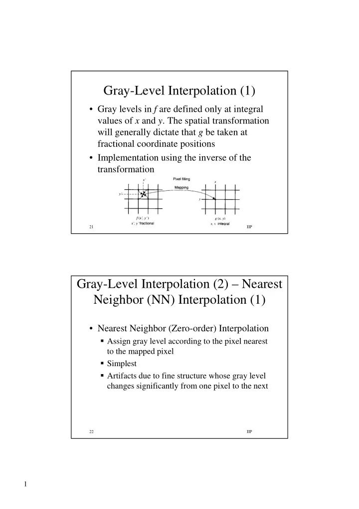
Gray-Level Interpolation (1)

• Gray levels in f are defined only at integral

values of x and y. The spatial transformation will generally dictate that g be taken at fractional coordinate positions

• Implementation using the inverse of the

transformation

IIP 22

Gray-Level Interpolation (2) – Nearest Neighbor (NN) Interpolation (1)

• Nearest Neighbor (Zero-order) Interpolation

Assign gray level according to the pixel nearest to the mapped pixel Simplest Artifacts due to fine structure whose gray level changes significantly from one pixel to the next

2

IIP 23

Gray-Level Interpolation (3) – Bilinear Interpolation (1)

• Bilinear (First order ) Interpolation

Better than zero order with moderate increase in programming complexity

• is known at the vertices of the unit square

and we wish to interpolate the value of at an arbitrary point inside the square We do that by fitting a hyperbolic paraboloid defined by the bilinear equation through the four known values at the vertices. The coefficients are chosen so that fits the values at the vertices

d cxy by ax y x f + + + = ) , (

( , ) f x y ( , ) f x y ( , ) f x y

IIP 24

Gray-Level Interpolation (4) – Bilinear Interpolation (2)

• A simple algorithm for bilinear interpolation:

[ ] [ ] [ ]

linearly interpolate between upper two points ( ,0) (0,0) (1,0) (0,0) and similarly for lower two points ( ,1) (0,1) (1,1) (0,1) and then vertically ( , ) ( ,0) ( ,1) ( ,0) yielding ( , ) (1 f x f x f f f x f x f f f x y f x y f x f x f x y f = + − = + − = + − =[

] [ ] [ ]

,0) (0,0) (0,1) (0,0) (1,1) (0,0) (0,1) (1,0) (0,0) bilinear f x f f y f f f f xy f − + − + + − − +

3

IIP 25

Gray-Level Interpolation (5)

• Zero (NN) vs. first order interpolation

first zero

Castleman, 1996

IIP 26

Geometric Operations – Applications

• Geometric calibration (removal of camera-

induced geometric distortion, e.g., airborne & satellite)

• Image registration (of similar images before

comparison due, e.g., to different viewing angles)

• Image rectification (transformation of non-

rectangular pixel coordinates to rectangular coordinates)

• Image morphing (transform one object gradually

into another)

• …

4

IIP 27

Image Rectification – Example

• Fish-eye lens

for robots

Castleman, 1996

IIP 28

Image Morphing – Example

(a) initial (b) 40% points (c) 70% points (d) final

Castleman, 1996

5

IIP 29

Image Enhancement in the Spatial Domain by Filtering

• Reminder: procedures (operators) operating
• n pixels
• Performed by moving a mask (also called

window, filter, template), centered at the current pixel, over the image and applying the

• perator on mask’s pixels to obtain the
• perator value at the current pixel. Practically,

the operator is specified by the mask coefficients

IIP 30

Image Enhancement by Filtering – The Mechanism (1)

x mask and 2 1, 2 1, , nonnegative integers (i.e., mask of odd size) m n m a n b a b = + = + ( 1, 1) ( 1, 1) ( 1,0) ( 1, ) ... (0,0) ( , ) ... (1,0) ( 1, ) (1,1) ( 1, 1) and linear filtering of an image of size x with a filter mask of size x is ( R w f x y w f x y w f x y w f x y w f x y f M N m n g x = − − − − + − − + + + + + + + + , ) ( , ) ( , ) also called "convolution of a mask with an image"

a b s a t b

y w s t f x s y t

=− =−

= + +

∑ ∑

6

IIP 31

Image Enhancement by Filtering – The Mechanism (2)

• Or for 3x3 mask, the response is
• What about the edges?

1) Limit range 2) Partial mask 3) Padding

9 1 i i i

R w z

=

= ∑

IIP 32

Smoothing (1)

• Used for:

Blurring (removal of small details or bridging small gaps in lines or curves) Noise reduction (however affects also edges)

• Implemented by averaging gray levels

within the mask

( , ) ( , ) ( , ) ( , )

a b s a t b a b s a t b

w s t f x s y t g x y w s t

=− =− =− =−

+ + = ∑ ∑

∑ ∑

7

IIP 33

Smoothing (or Low-Pass Filter) (2)

• 1D image example

[ ] [ ] [ ] 3

1 * 6,26,8,9 10,16,22,2 3,7,11,11, b * a 3 1 * 1,1,1 b 4,9,9,8,9 3,4,4,3,3, a = = =

edge~0.55 smoothed edge~0.09 low-pass filter

IIP 34

Smoothing (3)

weighted average mask average mask

8

IIP 35

Smoothing (4)

Gonzalez & Woods, 2002

IIP 36

Smoothing (5)

Gonzalez & Woods, 2002

9

IIP 37

Median Filter (1)

One of order-statistics filter Neighborhood (local) operation Nonlinear Slow process due to ranking

IIP 38

Median Filter (2)

• Simple example

20 10 15 20 250 15 5 20 10

brightness values in a 3x3 image section 5 10 10 15 15 20 20 20 250 1st 2nd 3rd 4th 5th 6th 7th 8th 9th ^ ^ ^

• min. median max.

brightness values in ascending order (in comparison to average of 40)

10

IIP 39

Median Filter (3)

• Example

1 2 3 4 5 1 2 3 4 5 6 7 8 9 10 1 2 3 4 1 2 3 4 5 6 7 8 9 10

1D image (edge + sinusoid) filtered with 3x1 median

IIP 40

Median Filter (4)

Gonzalez & Woods, 2002