SLIDE 7 7
A more careful analysis
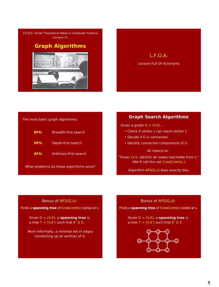
AFS(G,s):
Put s into bag While bag is not empty: Pick arbitrary tile v from bag If v is “unmarked”: “Mark” v For each neighbor w of v: Put w into bag
Every time a bunch of tiles is added to bag, it’s because some vertex v just got marked. In this case, we add deg(v) tiles to the bag. Each iteration through loop removes 1 tile. ∴ AFS halts after ≤ 2|E| many iterations. ∴ total number of tiles that ever enter the bag is
= 2|E| ≤
we forgot about this line
+1
When a tile w is added to the bag, it gets there “because of” a neighbor v that was just marked. (Except for the initial s .) Let’s actually record this info on the tile, writing v→w . Meaning: “We want to keep exploring from w. By the way, we got to w from v.” (And we’ll write ⊥→s initially.) AFS(G,s):
Put s into bag While bag is not empty: Pick an Arbitrary tile v from bag If v is “unmarked”: “Mark” v For each neighbor w of v: Put w into bag
AFS(G,s):
Put ⊥→s into bag While bag is not empty: Pick an Arbitrary tile p→v from bag If v is “unmarked”: “Mark” v For each neighbor w of v: Put v→w into bag
AFS(G,s):
Put ⊥→s into bag While bag is not empty: Pick an Arbitrary tile p→v from bag If v is “unmarked”: “Mark” v and record parent(v) := p For each neighbor w of v: Put v→w into bag
1 5 6 7 8 2 3 4
✓
2 5 2 5 2 3 6
✓ ✓
AFS(G,s):
Put ⊥→s into bag While bag is not empty: Pick an Arbitrary tile p→v from bag If v is “unmarked”: “Mark” v and record parent(v) := p For each neighbor w of v: Put v→w into bag
1 5 6 7 8 2 3 4
1→2 1→5 6→2 6→5 7→2 7→3 7→6
✓
⊥
✓ ✓
parent