Graph Algorithms Graph Algorithms g Undirected: edge ( u , v ) = ( - PowerPoint PPT Presentation

Graphs � Graph G = ( V , E ) » V = set of vertices Introduction to Algorithms Introduction to Algorithms » E = set of edges ⊆ ( V × V ) E f d ( V V ) � Types of graphs Graph Algorithms Graph Algorithms g » Undirected: edge ( u , v ) = ( v , u ); for all v , ( v , v ) ∉ E (No self » Undirected: edge ( u v ) = ( v u ); for all v ( v v ) ∉ E (No self loops.) » Directed: ( u , v ) is edge from u to v , denoted as u → v . Self loops CSE 680 are allowed. ll d Prof. Roger Crawfis » Weighted: each edge has an associated weight, given by a weight function w : E → R . » Dense: | E | ≈ | V | 2 . » Sparse: | E | << | V | 2 . 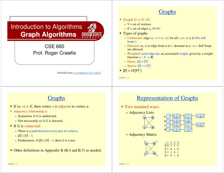� | E | = O (| V| 2 ) | E | O (| V| 2 ) Partially from io.uwinnipeg.ca/~ychen2 graphs-1 - 2 Graphs Representation of Graphs � If ( u , v ) ∈ E , then vertex v is adjacent to vertex u . � Two standard ways. � Adjacency relationship is: » Adjacency Lists. j y » Symmetric if G is undirected. b d c a a b » Not necessarily so if G is directed. a c b � If G is connected: d d a b b c c d d a c » There is a path between every pair of vertices. » Adjacency Matrix. » Adjacency Matrix » | E | ≥ | V | – 1. | E | ≥ | V | 1 » Furthermore, if | E | = | V | – 1, then G is a tree. 1 2 1 2 3 4 a b 1 0 1 1 1 1 0 1 1 1 2 1 0 1 0 � Other definitions in Appendix B (B.4 and B.5) as needed. 3 1 1 0 1 c d 3 3 4 4 4 1 0 1 0 4 1 0 1 0 graphs-1 - 3 graphs-1 - 4

Adjacency Lists Storage Requirement � Consists of an array Adj of | V | lists. � For directed graphs: � One list per vertex. » Sum of lengths of all adj. lists is p ∑ out-degree( v ) = | E | � For u ∈ V , Adj [ u ] consists of all vertices adjacent to u . v ∈ V No. of edges leaving v a a b b b b d d c c a a » Total storage: Θ (| V| + | E| ) c b If weighted, store weights also in � For undirected graphs: d c c d adjacency lists. dj li t » Sum of lengths of all adj. lists is d ∑ degree( v ) = 2| E | a b b d c a v ∈ V V No. of edges incident on v. Edge ( u , v ) is incident a c b on vertices u and v . » Total storage: Θ (| V| + | E| ) d a b c c d d a c graphs-1 - 5 graphs-1 - 6 Pros and Cons: adj list Adjacency Matrix � | V | × | V | matrix A . � Pros � Number vertices from 1 to | V | in some arbitrary manner. » Space-efficient, when a graph is sparse. | | y » Can be modified to support many graph variants. � A is then given by: � Cons ∈ ⎧ 1 if ( i , j ) E = = ⎨ ⎨ A A [ [ i i , j j ] ] a » Determining if an edge ( u , v ) ∈ G is not efficient. ij ⎩ 0 otherwise • Have to search in u ’s adjacency list. Θ (degree( u )) time. 1 1 2 2 • Θ ( V ) in the worst case Θ ( V ) in the worst case. 1 2 3 4 1 2 3 4 1 2 3 4 1 2 3 4 a a b b a b b 1 0 1 1 1 1 0 1 1 1 2 1 0 1 0 2 0 0 1 0 3 1 1 0 1 3 0 0 0 1 c c d d c c d d 4 3 4 4 1 0 1 0 3 4 0 0 0 0 A = A T for undirected graphs. graphs-1 - 7 graphs-1 - 8

Space and Time Some graph operations Some graph operations � Space: Θ ( V 2 ) . » Not memory efficient for large graphs. adjacency matrix adjacency lists � Time: to list all vertices adjacent to u : Θ ( V ) . � Time: to determine if ( u , v ) ∈ E : Θ ( 1 ) . O(e) insertEdge g O(1) ( ) � Can store weights instead of bits for weighted graph. isEdge O(e) O(1) #successors? O(e) O(V) #predecessors? d O(E) O(E) O(V) graphs-1 - 9 graphs-1 - 10 traversing a graph Graph Definitions � Path » Sequence of nodes n 1 , n 2 , … n k S q 1 , 2 , k » Edge exists between each pair of nodes n i , n i+1 ny bos » Example » Example • A, B, C is a path dc dc la la chi hi atl atl Where to start? Will all vertices be visited? Will all vertices be visited? How to prevent multiple visits? graphs-1 - 11 graphs-1 - 12

Graph Definitions Graph Definitions � Path � Cycle » Sequence of nodes n 1 , n 2 , … n k S q 1 , 2 , » Path that ends back at starting node g k » Edge exists between each pair of nodes n i , n i+1 » Example » Example » Example • A, E, A , , • A, B, C is a path • A, E, D is not a path , , p graphs-1 - 13 graphs-1 - 14 Graph Definitions Graph Definitions � Cycle � Reachable » Path that ends back at starting node g » Path exists between nodes � Connected graph » Example • A, E, A , , » Every node is reachable from some node in graph » Every node is reachable from some node in graph • A, B, C, D, E, A � Simple path S p e pat » No cycles in path � Acyclic graph � Acyclic graph » No cycles in graph Unconnected graphs graphs-1 - 15 graphs-1 - 16

Graph-searching Algorithms Breadth-first Search � Input: Graph G = ( V , E ) , either directed or undirected, � Searching a graph: and source vertex s ∈ V . » Systematically follow the edges of a graph � Output: O to visit the vertices of the graph. » d [ v ] = distance (smallest # of edges, or shortest path) from s to v , � Used to discover the structure of a graph. for all v ∈ V . d [ v ] for all v ∈ V . d [ v ] = ∞ if v is not reachable from s. if v is not reachable from s. � Standard graph-searching algorithms. » π [ v ] = u such that ( u , v ) is last edge on shortest path s v . » Breadth-first Search (BFS). • u is v ’s predecessor. » Builds breadth-first tree with root s that contains all reachable B ild b dth fi t t ith t th t t i ll h bl » Depth-first Search (DFS). D h fi S h (DFS) vertices. graphs-1 - 17 graphs-1 - 18 Breadth-first Search BFS for Shortest Paths � Expands the frontier between discovered and Finished undiscovered vertices uniformly across the breadth Discovered Discovered 1 1 of the frontier. S 1 Undiscovered 1 » A vertex is “discovered” the first time it is encountered d during the search. i th h » A vertex is “finished” if all vertices adjacent to it have 2 been discovered been discovered. 3 3 3 3 � Colors the vertices to keep track of progress. 2 2 3 » White – Undiscovered. » White – Undiscovered 1 1 S S S S 2 1 » Gray – Discovered but not finished. 1 2 » Black Finished. » Black – Finished 3 2 3 graphs-1 - 19 graphs-1 - 20

BFS(G,s) Example (BFS) 1. for each vertex u in V[G] – {s} do color [ u ] ← white do color [ u ] ← white 2 2 initialization d [ u ] ← ∝ 3 π [ u ] ← nil 4 white: undiscovered color[ s ] ← gray 5 gray: discovered d[ s ] ← 0 black: finished 6 access source s r s t u π [ s ] ← nil 7 Q ← Φ ∞ ∞ ∞ 8 0 Q : a queue of discovered 9 enqueue( Q ,s) vertices 10 while Q ≠ Φ color[ v ]: color of v d[ v ]: distance from s to v do u ← dequeue(Q) 11 π [ u ]: predecessor of v 12 12 for each v in Adj[ u ] for each v in Adj[ u ] ∞ ∞ ∞ ∞ 13 do if color[ v ] = white then color[ v ] ← gray 14 v w x y d [ v ] ← d [ u ] + 1 d [ v ] ← d [ u ] + 1 15 15 π [ v ] ← u 16 17 enqueue( Q , v ) Q: s color[ u ] ← black 18 0 0 graphs-1 - 21 graphs-1 - 22 Example (BFS) Example (BFS) r r s t u s t u ∞ ∞ ∞ 2 1 0 1 0 ∞ ∞ ∞ ∞ ∞ 2 1 1 v w x y v w x y Q: w r Q: r t x 1 1 1 1 1 2 2 1 2 2 graphs-1 - 23 graphs-1 - 24

Example (BFS) Example (BFS) r s r s t u t u ∞ 2 2 0 0 3 1 1 ∞ ∞ 2 2 2 1 2 1 v w v w x y x y Q: t x v Q: x v u 2 2 2 2 2 2 2 2 3 2 2 3 graphs-1 - 25 graphs-1 - 26 Example (BFS) Example (BFS) r r s t u s t u 2 2 1 0 3 1 0 3 2 2 2 1 3 2 1 3 v w x y v w x y Q: v u y Q: u y 2 3 3 2 3 3 3 3 3 3 graphs-1 - 27 graphs-1 - 28

Example (BFS) Example (BFS) r s r s t u t u 2 2 0 3 0 3 1 1 2 3 2 3 2 1 2 1 v w v w x y x y Q: ∅ Q: y 3 3 graphs-1 - 29 graphs-1 - 30 Example (BFS) Analysis of BFS � Initialization takes O (| V| ) . � Traversal Loop » After initialization, each vertex is enqueued and dequeued at most r s t u once, and each operation takes O (1) . So, total time for queuing is 2 O (| V| ) . (| | ) 1 0 3 » The adjacency list of each vertex is scanned at most once. The sum of lengths of all adjacency lists is Θ (| E| ) . � Summing up over all vertices > total running time of BFS � Summing up over all vertices => total running time of BFS 2 2 1 3 is O (| V| + |E| ), linear in the size of the adjacency list representation of graph. v w x y BF Tree graphs-1 - 31 graphs-1 - 32